Deep Residual Learning for Image Recognition

Presented by

Hanzhen Yang, Jing Pu Sun, Ganyuan Xuan, Yu Su, Jiacheng Weng, Keqi Li, Yi Qian, Bomeng Liu

Modeling

Convolutional deep neural network is constructed by simply stacking many layers together. Such formulation of deep network exists two problems during training: 1) vanishing gradient problem; 2) degradation of accuracy [1]. In this section, detailed explanation of these two problems and corresponding solutions are discussed.

Vanishing / Exploding Gradient

Deep neural networks are trained using back propagation. The error gradient with respect to weight parameters at shallower layers can be expressed as a chain rule expansion of parameters at deeper layers. When a network has large number of layers, the gradient tends to vanish or explode during back propagation.

Consider a simple example of feedforward neural network with only one neuron at each layer as shown in figure [XX1].

Figure [XX1]: simple feedforward neural network with one neuron at hidden layers

The error gradient of weight [math]\displaystyle{ w_1 }[/math] can be expressed as:

[math]\displaystyle{ \frac{\partial Err}{\partial w_1} = \frac{\partial Err}{\partial \hat{y}}\frac{\partial \hat{y}}{\partial x_3}\frac{\partial x_3}{\partial x_2}\frac{\partial x_2}{\partial w_1} \\ \ \ \ \ \ \ \ \ = \frac{\partial Err}{\partial \hat{y}} \cdot w_3 \cdot \sigma'(x_2 w_2) \cdot w_2 \cdot \sigma'(x_1 w_1) \cdot x_1 }[/math]

The activation function at each neuron is commonly selected to be Relu to avoid vanishing gradient when performing differentiation [REF]. When weight [math]\displaystyle{ w_3 }[/math] and [math]\displaystyle{ w_2 }[/math] are less than 1, the error gradient with respect to [math]\displaystyle{ w_1 }[/math] can be small due to multiplication of small numbers (a.k.a. vanishing gradient). When [math]\displaystyle{ w_3 }[/math] and [math]\displaystyle{ w_2 }[/math] are greater than 1, the error gradient with respect to [math]\displaystyle{ w_1 }[/math] can be large (a.k.a. exploding gradient). Both of these situations increase the difficulty of training.

degradation of accuracy

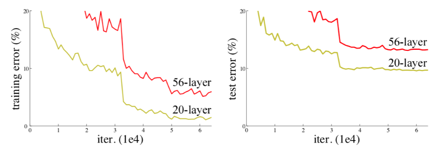
From empirical results, neural networks with stochastic gradient descent has difficulty optimizing the unnecessary weight to identity [1]. That is, adding more layers to a optimized model can increase the training error which contradicts to common understanding of neural networks. Figure [XX2] shows the comparison between training error of shallow and deep networks.

Figure [XX2]: Training error (left) and test error (right) on CIFAR-10 with 20-layer and 56-layer “plain” networks [1]

Assuming the deeper network is capable of training identity on the extra layers, it should produce training error no larger than the shallower network. This suggests that convolutional formulation of neural networks has difficulty of training identity.

Solution

To resolve vanishing / exploding gradient and degradation of accuracy, residual network (Resnet) is proposed by K. He, etc [1]. The mathematical explanation are discussed in this section.

FIgure [XX3] shows a representation of Resnet building block. The main change of the Resnet is to include a short-cut that passes information directly from shallower layer to deeper layer.

Figure [XX3]: Residual learning: a building block [1]

Table [XX1] illustrates the comparison of training identity in a Resnet and a convolutional neural network. Relu operation of x is denoted as [math]\displaystyle{ f(x) }[/math]. Assuming x1 is the output of a previous building block, thus [math]\displaystyle{ ReLU(x_1) = x_1 }[/math]. In order to train identity in a Resnet building block, weight matrix need to be trained to 0 instead of I which is assumed to be easier[1]. This is further proven in the Experiment / Results section.

Table [XX1]: Comparison between no short-cut and with short-cut formulation

	Expression of [math]\displaystyle{ x_3 }[/math]	Condition for [math]\displaystyle{ x_1 = x_3 }[/math]
No short-cut	[math]\displaystyle{ x_2 = f(W_2 \cdot f(W_1x_1)) }[/math]	[math]\displaystyle{ W_1 = W_2 = I }[/math]
With short-cut	[math]\displaystyle{ x_2 = f(W_2 \cdot f(W_1x_1)) + x_1 }[/math]	[math]\displaystyle{ W_1 = 0 }[/math] or [math]\displaystyle{ W_2 = 0 }[/math]

The formulation of Resnet also addresses the vanishing / exploding gradient problem. According to figure [XX3], we denote [math]\displaystyle{ F(x_1, W_1^{'}) = W_2 f(W_1x_1) }[/math] where [math]\displaystyle{ W_1^{'} }[/math] is the equivalent weight parameters, then [math]\displaystyle{ x_2 = x_1 + F(x_1, W_1^{'}) }[/math]. To generalize the index, we obtain the following equations [3]:

[math]\displaystyle{ y_l = x_l + F(x_l, W_l^{'}) \\ x_{l+1} = f(y_l) }[/math]

Recursively, we can express x at any deeper layer L using information from shallower layer as following [3]:

[math]\displaystyle{ x_L = x_l + \sum_{i=1}^{L-1} F(x_i, W_i^{'}) }[/math]

By rearranging equation above, and differentiating with chain rule, the following expression is obtained [3]:

[math]\displaystyle{ \frac{\partial Err}{\partial x_l} = \frac{\partial Err}{\partial x_L} \frac{\partial x_L}{\partial x_l} = \frac{\partial Err}{\partial x_L} (1+ \frac{\partial }{\partial x_l} \sum_{i=1}^{L-1} F(x_i, W_i^{'})) }[/math]

This suggests that the gradient at shallower layer [math]\displaystyle{ l }[/math] sees information directly from deeper layer [math]\displaystyle{ L }[/math]. To make the error gradient at layer [math]\displaystyle{ l }[/math] vanish, the derivative term of [math]\displaystyle{ \sum F }[/math]must be equal to -1 which is very difficult to achieve in a batch learning process [3]. Since error gradient with respect to [math]\displaystyle{ x_l }[/math] is part of back propagation process, preventing vanishing gradient wrt. [math]\displaystyle{ x_l }[/math] can effectively prevent vanishing gradient of [math]\displaystyle{ W_{l-1} }[/math].

Intuition of Resnet

Figure [XX4] shows a interesting way of understanding Resnet. By expanding a simple Resnet with 3 building block, a graph with all possible path of information is constructed. Therefore, the Resnet can also be seen as a majority voting process.

Figure [XX4]: Understand Resnet as a majority voting process [4]