Bag of Tricks for Efficient Text Classification
- WORK IN PROGRESS*
Introduction and Motivation
Text Classification is utilized by millions of web users on a daily basis. An example of an application of text classification is web search and content ranking. When a user searches a specific word that best describes the content they are looking for, text classification helps with categorizing the appropriate content.
Neural networks have been utilized more recently for Text-Classifications and demonstrated very good performances. However, it is slow at both training and testing time, therefore limiting their usage for very large datasets. The motivation for this paper is to determine whether a simpler text classifier, which is inexpensive in terms of training and test time, can approximate the performance of these more complex neural networks.
The authors suggest that linear classifiers are very effective if the right features are used. The simplicity of linear classifiers allows a model to be scaled to very large data set while maintaining its good performance.
The basis of the analysis for this paper was applying the classifier fastText to the two tasks: tag predictions and sentiment analysis, and comparing its performance and efficiency with other text classifiers. The paper claims that this method “can train on billion word within ten minutes, while achieving performance on par with the state of the art.”
Background
- PLACEHOLDER: we should look at when this
Natural-Language Processing
Natural Language Processing (NLP) is concerned with being able to process large amounts of natural language data, involving speech recognition, natural language understanding, and natural-language generation. Text understanding involves being able to understand the explicit or implicit meaning of elements of text such as words, phrases, sentences, and paragraphs, and making inferences about these properties of texts (Norvig, 1987). One of the main topics in NLP is text classification, which is assigning predefined categories to free-text documents, with research ranging in this field from designing the best features to choosing the best machine learning classifiers (Zhang et al. 2016).
Traditionally, techniques for text classification are based on simple statistics on words. (Talk about linear classifiers? typical models?)
With the advancement of deep learning and the availability of large data sets, methods of handling text understanding using deep learning techniques have become available in recent years. (talk about deep learning models briefly)
- Briefly describe the difference between NLP and text-mining. Maybe comment later about whether fastText accomplishes NLP.
Char-CNN
Char-CRNN
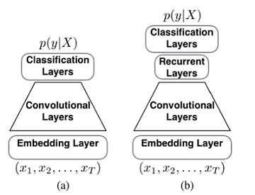
A chactacter-level convolutional neural network (CRNN) is a a convolutional neural network (CNN) with a recurrent layer on top. A recurrent layer can efficiently capture long-term dependencies, therefore a model with only a very small number of convolutional layers is needed.
The recurrent layer consists of a recursive function [math]\displaystyle{ f }[/math] which takes as input one input vector and the previous hidden state, and returns the new hidden state [math]\displaystyle{ h_t = f(x_t, h_{t-1}) }[/math], where [math]\displaystyle{ x_t \epsilon \mathbb{R}^d }[/math] is one time step from the input sequence [math]\displaystyle{ (x_1, x_2, ,..., x_T) }[/math].
 Graphical illustration of (a) a CNN and (b) proposed CRNN for character-level document classification
Source: [Xiao and Cho2016] Yijun Xiao and Kyunghyun Cho. 2016. Efficient character-level document classification by combining convolution and recurrent layers. arXiv preprint arXiv: 1602.00367.
VDCNN
Model
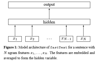
Model Architecture of fastText
Traditionally, text classification methods were centered around linear classifiers. Linear classifier is limited by its inability to share parameters among features and classes. As a result, classes with very few examples will often get classified in a large output field. The authors of this paper will attempt to improve on the performance of linear classifiers with the key features of rank constraint and fast loss approximation. Before we get into that, we must better understand the idea of model training of linear classifiers.
Consider each text and each label as a vector in space. The model is training the coordinates of the text vector, in order for the text vector to be close to the vector of its associated label. The text vector and its label vector is inputted into the softmax function, which returns a score. The score is then normalized across the score for that same text with every other possible label. The result is the probability that the text will have its associated label. Then stochastic gradient descent algorithm is used to keep updating the coordinates until the probability of correct label for every text is maximized. This is clearly computationally expensive, as the score for every possible label in the training set must be computed for a text.
A softmax function returns a probability that a text is associated with label j, with K labels in the training set is:
[math]\displaystyle{ P(y=j | \mathbf{x}) = \dfrac{e^{\mathbf{x}^T \mathbf{w}_j}}{\sum_{k=1}^K e^{\mathbf{x}^T \mathbf{w}_k}} }[/math] ,where x represents the text vector and w represents the label vector.
Now let’s look at the improved method of linear classifiers with a rank constraint and fat loss approximation. Refer to the image below.
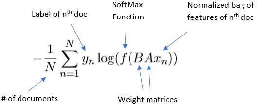
Using the weight matrices, the ngram features of the input are first looked up to find word representations, then averaged into hidden text representation. It is then fed to a linear classifier. Finally, the softmax function is used to compute the probability distribution over the predefined classes. For a set of N documents, the model minimizes the negative log likelihood over the classes. The classifier trains on multiple CPUs using stochastic gradient descent and a linearly decaying learning rate.
Two changes that were applied in this model architecture are the hierarchical softmax function, which improves performance with a large number of classes, and the hashing trick to manage mappings of n-grams to local word order. These two nuances will be more thoroughly explained in the upcoming sections.
Softmax and Hierarchy Softmax
As mentioned above, the softmax function is used to compute the probability density over predefined classes. It calculates the probability of [math]\displaystyle{ y_n }[/math] as each possible class and outputs probability estimates for each class. Due to the nature of the softmax function, the denominator serves to normalize the probabilities, allowing a single [math]\displaystyle{ y_n }[/math] to receive probabilities for each label, where these probabilities sum to one. This provides a means to choose the highest probability as the corresponding label for [math]\displaystyle{ y_n }[/math].
However, the softmax function does have a computational complexity of [math]\displaystyle{ O(Kd) }[/math] where [math]\displaystyle{ K }[/math] is the number of classes and [math]\displaystyle{ d }[/math] is the number of dimensions in the hidden layer of the neural network. This is due to the nature of the softmax function since each function calculation requires normalizing the probabilities over all potential classes. This runtime is not ideal when the number of classes is large, and for this reason a hierarchical softmax function is used. We can see the differences in computational efficiency in the following set-up for hierarchical softmax.
Suppose we have a binary tree structure based on Huffman coding for the softmax function, where each node has at most two children or leaves. Huffman coding trees provide a means to optimize binary trees where the classes with lowest frequencies are placed deeper into the tree and the highest frequency classes are placed near the root of the tree, which minimizes the path for more frequently labelled classes. Huffman coding trees are efficient since computational runtime is reduced to [math]\displaystyle{ O(d \log_2(K)) }[/math].
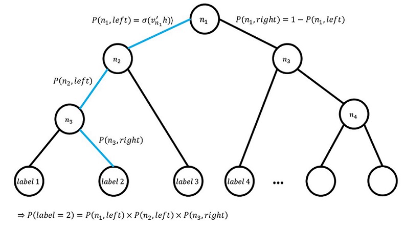
A probability for each path, whether we are travelling right or left from a node, is calculated. This is done by applying the sigmoid function to the product of the output vector [math]\displaystyle{ v_{n_i} }[/math] of each inner node [math]\displaystyle{ n }[/math] and the output value of the hidden layer of the model, [math]\displaystyle{ h }[/math]. The idea of this method is to represent the output classes as the leaves on this tree and a random walk then assigns probabilities for these classes based on the path taken from the root of the tree. The probability of a certain class is then calculated as:
where [math]\displaystyle{ n }[/math] represents the leaf node that a class is located on with depth [math]\displaystyle{ l+1 }[/math] and [math]\displaystyle{ n_1, n_2, …, n_l }[/math] represents the parent nodes of that leaf
In the below figure, we can see an example of a binary tree for the hierarchical softmax model. An example path from root node [math]\displaystyle{ n_1 }[/math] to label 2 is highlighted in blue. In this case we can see that each path has an associated probability calculation and the total probability of label 2 is in line with the class probability calculation above.
Note that during the training process, vector representations for inner nodes, [math]\displaystyle{ v_{n_i} }[/math], are updated by introducing an error function, [math]\displaystyle{ Err }[/math] and deriving the error function to obtain the following:
We can use this to update the vector values with the following:
N-Gram, Bag of Words, and TFIDF
Bag of Words
Bag of word is an algorithm for simplifying a text dataset by counting how many times a word appears in a document. The n most frequent words are extracted from the training subset to be used as the “dictionary” for the testing set. This dictionary allow us to compare document for document classification and topic modeling. This is one of the method that the authors used for preparing text for input. Each vector of word count is normalized such that all the elements of the vector adds up to one (taking the frequency percentage of the word). If these frequencies exceeds a certain level it will activate nodes in neural network and influence classification.
The main weakness of bag of word is that it losses information due to it being single word and invariant to order. We will demonstrate that shortly. Bag of word will also have high error percentage if the training set does not include the entire dictionary of the testing set.
N-Gram
N-gram is another model for simplifying text replication by storing n-local words adjacent to the initial word (or character, N-gram can be character based. Each words in the document is read one at a time just like bag of words, however a certain range of its neighbors will also be scanned as well. This range is known as the n-grams. Compared to bag of words, any N over 1 (noted as Unigram) will contain more information than bag of words.
In the picture above, it gives an example of a Unigram (1-gram) which is the absolute simplest possible version of this model. Unigram does not consider previous words and just chooses random words based on how common they are in general. It also shows a Bigram (2-gram), where the previous word is considered. Trigram would consider the previous two words, etc etc. Up to N-grams, where it considers N-1 previous words.
Let a sentence be denoted as a product of words 1 to word n, [math]\displaystyle{ \omega_1^n = \omega_1 \cdots \omega_n }[/math] . By probabilities properties, we can model the probability of the word sequence 1 with Bigram as [math]\displaystyle{ P(\omega_1^n) =P( \omega_1) P( \omega_2 | \omega_1) P( \omega_3 | \omega_1^2) \cdots P( \omega_n | \omega_1^{n-1}) }[/math] . For example, take the sentence, "How long can this go on?" We can model it as followed:
P(How long can this go on?”)= P(How)P(long | How)P(can | long)P(this | can)P(go | this)P(on | go)P(? | on)
Going back to the chain event probability. We can reduce the above equation as the Product of the conditional probabilities as follows for the Bigram case:
[math]\displaystyle{ P(\omega_1^n) = \prod_{k=1}^n P(\omega_k | \omega_{k-1} ) }[/math].
We can generalize this to the stronger case for N-th gram as:
[math]\displaystyle{ P(\omega_1^n) = \prod_{k=1}^n P(\omega_k | \omega_{k-(N-1)}^{k-1} ) }[/math].
The weakness with N-gram is that many times local context does not provide any useful predictive clues. For example, if you want the model to learn plural usage of the following sentence:
         The woman who lives on the fifth floor of the apartment is pretty.
         The women who lives on the fifth floor of the apartment are pretty.
You will need to use 11-th gram and it is very unfeasible for ordinary machines. Which brings us to the next problem, as N increases, the predictive power of the model increases, however the number of parameters required grows exponentially with the number of words prior context.
BoW, Unigram, Bigram Example
An example of this is found in the below example
A = “I love apple”
B = “apple love I”
C = “I love sentence”
| A | B | C | |
| I | 1 | 1 | 1 |
| love | 1 | 1 | 0 |
| apple | 1 | 1 | 0 |
| sentence | 0 | 0 | 1 |
Notice how A and B are the same vector. This is just like bag of word and the aforementioned problem of order does not matter!
| A | B | C | |
| I love | 1 | 0 | 1 |
| love apple | 1 | 0 | 0 |
| apple love | 0 | 1 | 0 |
| love i | 0 | 1 | 0 |
| love sentence | 0 | 0 | 1 |
Notice now, A and B are unique because bigram takes into consideration one space of local words. However, A and C also have similar elements, being I love. IF we were to further increase N in N-gram we will have an easier time in classifying the distinction between the two. Higher, the consequences of operating in higher dimension of N gram is that the run time will increase.
Feature Hashing
Feature hashing, aka hash trick, can be used in sentence classification which maps words to indices of an array or a matrix of fixed size by applying a hash function to features. The general idea is to map sentences from high dimensional features to lower dimensional to reduce the dimension of the input vector, and therefore, reduce the cost of storing large vectors.
A hash function is any function that maps an arbitrary array of keys to a list of fixed size. For example, consider a hash function [math]\displaystyle{ h }[/math] that maps features to the value of corresponding dictionary key.
| Key | Index |
|---|---|
| I | 0 |
| love | 1 |
| hate | 2 |
| cats | 3 |
| dogs | 4 |
| but | 5 |
| Mary | 6 |
In this case, [math]\displaystyle{ h(``\text{cats"}) = 3 }[/math]. Considering the sentence [math]\displaystyle{ `` \text{ I love cats, but Mary hate cats"} }[/math] and we will try to map it to a hash table with length of 7. After vectorizing it, we will have a list all words in that sentence [math]\displaystyle{ x = [``I", ``love", ``cats", ``but", ``Mary", ``hate", ``cats"] }[/math]. Consider the hashed feature map [math]\displaystyle{ \phi }[/math] is calculated by
[math]\displaystyle{ \phi_i^{h}(x) = \underset{j:h(x_j)=i}{\sum} 1 }[/math], where [math]\displaystyle{ i }[/math] is the corresponding index of the hashed feature map.
By applying hash function to each word of this sentence, we will get a list of returned indexes [0, 1, 3, 5, 6, 2, 3], and the corresponding hashed feature map will be
| 0 | 1 | 2 | 3 | 4 | 5 | 6 |
|---|---|---|---|---|---|---|
| 1 | 1 | 1 | 2 | 0 | 1 | 1 |
There are many choices of hash functions, but the general idea is to have a good hash function that distributes keys evenly across the hash table.
Hash collision happens when two distinct keys are mapped to the same indices. For example, for above example, if both "Mary" and "I" are mapped to the same index 0. The output hash table will then become:
| 0 | 1 | 2 | 3 | 4 | 5 | 6 |
|---|---|---|---|---|---|---|
| 2 | 1 | 1 | 2 | 0 | 1 | 0 |
In order to get an unbiased estimate, the paper uses a signed hash kernel as introduced in Weinberger et al.2009, which introduces another hash function [math]\displaystyle{ \xi }[/math] to determine the sign of the return index. The hashed feature map [math]\displaystyle{ \phi }[/math] now becomes
[math]\displaystyle{ \phi_i^{h, \xi}(x) = \underset{j:h(x_j)=i}{\sum} \xi(x_j) \cdot 1 }[/math]
Consider if [math]\displaystyle{ \xi(``I") = 1 \text{ and } \xi(``Mary") = -1 }[/math], then our signed hash map now becomes:
| 0 | 1 | 2 | 3 | 4 | 5 | 6 |
|---|---|---|---|---|---|---|
| 0 | 1 | 1 | 2 | 0 | 1 | 0 |
Ideally, collisions will "cancel out", and therefore, achieve an unbiased estimate.
TF-IDF
For normal N-grams, word counts are used as features. However, another way that can be used to represent the features is called TFIDF, which is the short cut for term frequency–inverse document frequency. It represent the importance of a word to the document.
Term Frequency(TF) generally measures the times that a word occurs in a document. An Inverse Document Frequency(IDF) can be considered as an adjustment to the term frequency such that a word won't be deemed as important if that word is a generally common word, for example, "the".
TFIDF is calculated as the product of term frequency and inverse document frequency, generally expressed as [math]\displaystyle{ \mathrm{tfidf}(t,d,D) = \mathrm{tf}(t,d) \cdot \mathrm{idf}(t, D) }[/math]
In this paper, TFIDF is calculated in the same way as Zhang et al., 2015, with
- [math]\displaystyle{ \mathrm{tf}(t,d) = f_{t,d} }[/math], where [math]\displaystyle{ f_{t,d} }[/math] is the raw count of [math]\displaystyle{ t }[/math] for document [math]\displaystyle{ d }[/math].
- [math]\displaystyle{ \mathrm{idf}(t, D) = log(\frac{N}{| \{d\in D:t\in d \} |}) }[/math], where [math]\displaystyle{ N }[/math] is the total number of documents and [math]\displaystyle{ | \{d\in D:t\in d \} | }[/math] is the total number of documents that contains word [math]\displaystyle{ t }[/math].
Experiment
In this experiment fastText was compared on two classification problems with various other text classifiers.
The first classification problem being Sentiment Analysis, where it is compared to the existing text classifiers. Second, we evaluate fastText to a larger output space on a tag prediction dataset.
The Vowpal Wabbit library, written in C++ can also be used to implement our model. However, compared to this library, our tailored implementation is at least 2-5× faster in practice.
- Sentiment Analysis
- Tag Prediction
Tag prediction
Dataset
Scalability to large datasets is an important feature of a model. In order to test that, evaluation was carried the YFCC100M dataset which consists of approximately 100 million images containing captions, titles and tags for each. Here the, spotlight was on using fastText text classifier to predict the tags associated with each image without actually using the image itself, both rather the information associated with the image such as the title and caption of the image.
The methodology behind this classification problem was to remove the words and tags that occur less than 100 times and split the data into a train, validation and test set. The train set consists of approximately 90% of the dataset, the validation set consists of approximately 1%, and the test set of 0.5%. Table 4 shows an example of 5 items in the validation set with their Inputs (title and caption), Prediction (the tag class they are classified to) and Tags (real image tags), highlighting when the predicted class is in fact one of the tags.
| Input | Prediction | Tags |
|---|---|---|
| taiyoucon 2011 digitals: individuals digital photos from the anime convention taiyoucon 2011 in mesa, arizona. if you know the model and/or the character, please comment. | #cosplay | #24mm #anime #animeconvention #arizona #canon #con #convention #cos #cosplay #costume #mesa #play #taiyou #taiyoucon |
| 2012 twin cities pride 2012 twin cities pride parade | #minneapolis | #2012twincitiesprideparade #minneapolis #mn #usa |
| beagle enjoys the snowfall | #snow | #2007 #beagle #hillsboro #january #maddison #maddy #oregon #snow |
| christmas | #christmas | #cameraphone #mobile |
| euclid avenue | #newyorkcity | #cleveland #euclidavenue |
Removing infrequently occurring tags and words eliminates some noise and helps our model learn better. A script has been released explaining the breakup of the data. After cleaning, the vocabulary size is 297,141 and there are 312,116 unique tags. The precision of the model on the test set is reported at 1, meaning that all items classified to a tag did in fact belong to that class (Source: Wikipedia). (Need to figure out what this means, maybe move this line later on).
Baselines
A frequency-based approach which simply predicts the most frequent tag is used as a baseline.
The model we compare fastText to in tag prediction is Tagspace. It is similar to our model but is based on the WSABIE which predicts tags based on both images and their text annotations.
Tagspace is chosen as a comparison model because, similar to fastText, it is designed to predict tags. However, Tagspace predicts multiple tags, and the authors only evaluates prec@1, i,e, if their single tag prediction is correct or not. Hence, it does not fully compare the capabilities of the Tagspace model.
The Tagspace model is a convolution neural network, which predicts hashtags in semantic contexts of social network posts. For faster and better comparable performance, we consider the linear version of this model. (Linear version of Tagspace needs to be explained).
Results
| Model | prec@1 | Running time - Train | Running time - Test |
|---|---|---|---|
| Freq. baseline | 2.2 | - | - |
| Tagspace, h = 50 | 30.1 | 3h8 | 6h |
| Tagspace, h = 200 | 35.6 | 5h32 | 15h |
| fastText, h = 50 | 30.8 | 6m40 | 48s |
| fastText, h = 50, bigram | 35.6 | 7m47 | 50s |
| fastText, h = 200 | 40.7 | 10m34 | 1m29 |
| fastText, h = 200, bigram | 45.1 | 13m38 | 1m37 |
The above table presents a comparison of our fastText model to other baselines. The Precision-at-one(Prec@1) is the number of wins over the total number of search terms tried using the model.
We can see the frequency baseline has the lowest accuracy. On running fastText for 5 epochs and we compare it to Tagspace results. fastText with bigrams is also used and models are tested with 50 and 200 hidden layers. With 50 hidden layers, both fastText (without bigrams) and Tagspace performed similarly while fastText with bigrams performed better at 50 hidden layers than Tagspace did at 200. At 200 hidden layers, fastText performs better still and with bigrams, accuracy is improved. (Talk a little more about the accuracy the units and what it implies at the begining of accuracy section).
Finally, both the train and test times of our model performed significantly better than Tagspace which must compute the scores for each class. fastText on the other hand, has a fast inference which gives it an advantage for a large number of classes. In particular, test times for fastText are significantly faster than that of Tagspace.
Conclusion
The authors propose a simple baseline method for text classification that perform well on large-scale datasets. Word features are averaged together to represent sentences which is then fed to a linear classifier. The authors experiment and test their model fastText against other models with evaluation protocol similar to Zhang et al. (2015) for sentiment analysis and then evaluated on its ability to scale to large output on a tag prediction data set. fastText achieved comparable results in terms of accuracy and was found to train significantly faster.
Commentary and Criticism
Sources
Further Reading
- List of previous paper presentations in chronological order relating to text classification/fastText


