When can Multi-Site Datasets be Pooled for Regression? Hypothesis Tests, l2-consistency and Neuroscience Applications: Summary

This page is a summary for this ICML 2017 paper[1].

Introduction to some Basic Concepts and Issues

Regression Problems

Ridge and Lasso regression are powerful techniques generally used for creating parsimonious models in presence of a ‘large’ number of features. Here ‘large’ can typically mean either of two things[2]:

• Large enough to enhance the tendency of a model to overfit (as low as 10 variables might cause overfitting)
• Large enough to cause computational challenges. With modern systems, this situation might arise in case of millions or billions of features

Ridge Regression and Overfitting:

Ridge regression is commonly used in econometrics and thus machine learning. When fitting a model, unnecessary inputs or inputs with co-linearity might bring disastrously huge coefficients (with a large variance). Ridge regression performs L2 regularization, i.e. it adds a factor of sum of squared coefficients in the optimization objective. Thus, ridge regression optimizes the following.

• Objective = RSS + λ * (sum of square of coefficients)

Note that performing ridge regression is equivalent to minimizing RSS under the constraint that sum of squared coefficients is less than some function of λ, say s(λ). More specifically, ridge regression usually utilizes the method of cross-validation where we train the model on the training set using different values of λ and optimizing the above objective function. Then each of those model (each trained with different λ's) are tested on the validation set to evaluate their performance.

Lasso Regression and Model Selection:

LASSO stands for Least Absolute Shrinkage and Selection Operator. Lasso regression performs L1 regularization, i.e. it adds a factor of sum of absolute value of coefficients in the optimization objective. Thus, lasso regression optimizes the following.

• Objective = RSS + α * (sum of absolute value of coefficients)

1. α = 0: Same coefficients as simple linear regression
2. α = ∞: All coefficients zero (same logic as before)
3. 0 < α < ∞: coefficients between 0 and that of simple linear regression

A feature of Lasso regression is its job as a selection operator, i.e. it usually shrinks a part of coefficients to zero, while keeping the values of other coefficients. Thus it can be used in opting unnecessary coefficients out of the model.

Bias-Variance Trade-Off

The bias is error from erroneous assumptions in the learning algorithm. High bias can cause an algorithm to miss the relevant relations between features and target outputs (underfitting). The variance is error from sensitivity to small fluctuations in the training set. High variance can cause an algorithm to model the random noise in the training data, rather than the intended outputs (overfitting)[3]. Mean square error (MSE) is defined by (variance + squared bias). A thing to mention is the following theorem:

• For ridge regression, there exists a certain λ such that the MSE of coefficients calculated by ridge regression is smaller than that calculated by direct regression.

The Hypothesis Test

The hypothesis test to evaluate statistical power improvements (e.g., mean squared error) when running a regression model on a pooled dataset is discussed below.β corresponds to the coefficient vector (i.e., predictor weights), then the regression model is

• [math]\displaystyle{ min_{β} \frac{1}{n}\left \Vert y-Xβ \right \|_2^2 }[/math] ...... (1)

If k denotes the number of sites, a domain adaptation scheme needs to be applied to account for the distributional shifts between the k different predictors [math]\displaystyle{ \lbrace X_i \rbrace_{i=1}^{k} }[/math], and then run a regression model. If the underlying “concept” (i.e., predictors and responses relationship) can be assumed to be the same across the different sites, then it is reasonable to impose the same β for all sites. For example, the influence of CSF protein measurements on cognitive scores of an individual may be invariant to demographics. if the distributional mismatch correction is imperfect, we may define ∆ βi = βi − β∗ where i ∈ {1,...,k} as the residual difference between the site-specific coefficients and the true shared coefficient vector (in the ideal case, we have ∆ βi = 0)[1]. Therefore we derive the Multi-Site Regression equation ( Eq 2) where [math]\displaystyle{ \tau_i }[/math] is the weighting parameter for each site

• [math]\displaystyle{ min_{β} \displaystyle \sum_{i=1}^k {\tau_i^2\left \Vert y_i-X_iβ \right \|_2^2} }[/math] ......(2)

Separate Regression or Shared Regression ?

Since the underlying relationship between predictors and responses is the same across the different datasets ( from which its pooled), estimates of [math]\displaystyle{ \beta_i }[/math] across all k sites are restricted to be the same. Without this constraint , (3) is equivalent to fitting a regression separately on each site. To explore whether this constraint improves estimation, the Mean Square Error (MSE) needs to be examined[1]. Hence, using site 1 as the reference, and setting [math]\displaystyle{ \tau_1 }[/math] = 1 in (2) and considering [math]\displaystyle{ \beta*=\beta_1 }[/math],

• [math]\displaystyle{ min_{β} \frac{1}{n}\left \Vert y_1-X_1β \right \|_2^2 + \displaystyle \sum_{i=2}^k {\tau_i^2\left \Vert y_i-X_iβ \right \|_2^2} }[/math] .........(3)

To evaluate whether MSE is reduced, we first need to quantify the change in the bias and variance of (3) compared to (1).

Case 1: Sharing all [math]\displaystyle{ \beta }[/math]s

[math]\displaystyle{ n_i }[/math]: sample size of site i
[math]\displaystyle{ \hat{β}_i }[/math]: regression estimate from a specific site i.
[math]\displaystyle{ ∆β^T }[/math]:length kp vector

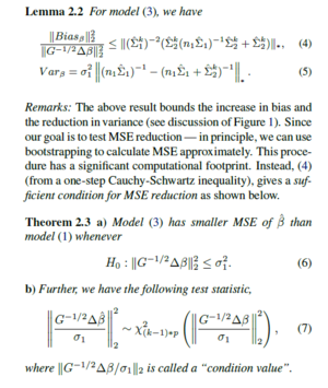
Lemma 2.2 bounds the increase in bias and reduction in variance. Theorem 2.3 is the author's main test result.Although [math]\displaystyle{ \sigma_i }[/math] is typically

unknown, it can be easily replaced using its site specific estimation. Theorem 2.3 implies that we can conduct a non-central [math]\displaystyle{ \chi^2 }[/math] distribution test based on the statistic.

Theorem 2.3 implies that the sites, in fact, do not even need to share the full dataset to assess whether pooling will be useful. Instead, the test only requires very high-level statistical information such as [math]\displaystyle{ \hat{\beta}_i,\hat{\Sigma}_i,\sigma_i }[/math] and [math]\displaystyle{ n_i }[/math] for all participating sites – which can be transferred without computational overhead.

Case 2: Sharing a subset of [math]\displaystyle{ \beta }[/math]s

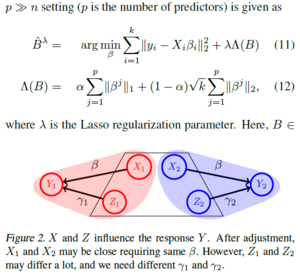
For example, socio-economic status may (or may not) have a significant association with a health outcome (response) depending on the country of the study (e.g., insurance coverage policies). Unlike Case 1, [math]\displaystyle{ \beta }[/math] cannot be considered to be the same across all sites. The model in (3) will now include another design matrix of predictors [math]\displaystyle{ Z\in R^{n*q} }[/math]and corresponding coefficients [math]\displaystyle{ \gamma_i }[/math] for each site i,

[math]\displaystyle{ min_{β,\gamma} \sum_{i=1}^{k}\tau_i^2\left \Vert y_i-X_iβ-Z_i\gamma_i \right \|_2^2 }[/math] ... (9)

While evaluating whether the MSE of [math]\displaystyle{ \beta }[/math] reduces, the MSE change in [math]\displaystyle{ \gamma }[/math] is ignored because they correspond to site-specific variables. If [math]\displaystyle{ \hat{\beta} }[/math]is close to the “true” [math]\displaystyle{ \beta* }[/math], it will also enable a better estimation of site-specific variables[1]

Sparse Multi-Site Lasso and High Dimensional Pooling

The effect of pooling multi-site data in the high-dimensional setting where the number of predictors p is much larger than number of subjects n studied ( p>>n).

[math]\displaystyle{ \ell2 }[/math]-consistency

---

MSE vs Sample Size plots

Sparse Multi-Site Lasso

In classical regression, [math]\displaystyle{ \ell2 }[/math] consistency properties are well known. Imposing the same [math]\displaystyle{ \beta }[/math] across sites works in (3) because we understand its consistency. In contrast, in the case where p>>n, one cannot enforce a shared coefficient vector for all sites before the active set of predictors within each site are selected — directly imposing the same leads to a loss of [math]\displaystyle{ \ell2 }[/math]-consistency, making follow-up analysis problematic. Therefore, once a suitable model for high-dimensional multi-site regression is chosen, the first requirement is to characterize its consistency.

Sparse Multi-Site Lasso Regression

The sparse multi-site Lasso variant is chosen because multi-task Lasso underperforms when the sparsity pattern of predictors is not identical across sites[4].The hyperparameter [math]\displaystyle{ \alpha\in [0, 1] }[/math] balances both L1 and L2 penalties;

• Larger [math]\displaystyle{ \alpha }[/math] weighs the L1 penalty more
• Smaller [math]\displaystyle{ \alpha }[/math] puts more weight on the grouping.

Similar to a Lasso-based regularization parameter, [math]\displaystyle{ \lambda }[/math] here will produce a solution path (to select coefficients) for a given [math]\displaystyle{ \alpha }[/math][1].

Experiments

There are 2 major experiments described:

1. Performing simulations to evaluate the hypothesis test from sparse multi-site Lasso
2. Pooling 2 Alzheimer's Disease datasets and examining the improvements in statistical power. This experiment was also done with the view of evaluating whether pooling is beneficial for regression and whether it yields tangible benefits in investigating scientific hypotheses[1].

Power and Type I Error

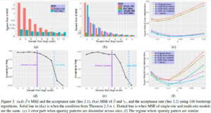
1. The first set of simulations evaluate Case 1 ( Sharing all β). The simulation are repeated 100 times with 9 different sample sizes. As n increases, both MSEs decrease ( two-site model and baseline single site model), and the test tends to reject pooling the multi-site data.
2. The second simulation set evaluates Case 2 variables ( Sharing subset of β). For small n, MSE of two-site model is much smaller than baseline, and as sample size increases this difference reduces. The test accepts with high probability for small n,and as sample size increases it rejects with high power.

SMS Lasso L2 Consistency

Two test cases where sparsity patterns are shared and not shared are considered separately, in 4 sites with n = 150 samples each and p = 400 features.

1. Few Sparsity Patterns Shared:6 shared features and 14 site-specific features (out of the 400) are set to be active in 4 sites. The chosen [math]\displaystyle{ \alpha }[/math]= 0:97 has the smallest error, across all [math]\displaystyle{ \lambda }[/math]s, thereby implying a better [math]\displaystyle{ \ell }[/math]2 consistency. [math]\displaystyle{ \alpha }[/math]= 0:97 discovers more always-active features, while preserving the ratio of correctly discovered active features to all the discovered ones.
2. Most Sparsity Patterns Shared: 16 shared and 4 site-specific features to be active among all 400 features were set.The proposed choice of [math]\displaystyle{ \alpha }[/math] = 0.25 preserves the correctly discovered number of always-active features. The ratio of correctly discovered active features to all discovered features increases here.

Combining AD Datasets from Multiple Sites

Pooling is evaluated empirically in a neuroscience problem regarding the combination of 2 Alzheimer's Datasets from different sources: ADNI (Alzheimer’s Disease Neuroimage Initiative) and ADlocal ( Wisconsin ADRC). The sample sizes are 318 and 156 respectively. Cerebrospinal fluid (CSF) protein levels are the inputs, and the response is hippocampus volume. Using 81 age-matched samples from each dataset, first domain adaptation is performed (using a maximum mean discrepancy objective as a measure of distance between the two marginals), and then transform CSF proteins from ADlocal to match with ADNI. The main aim is to evaluate whether adding ADlocal data to ADNI will improve the regression performed on ADNI. This is done by training a regression model on the ‘transformed’ ADlocal and a subset of ADNI data, and then testing the resulting model on the remaining ADNI samples.

• The results show that pooling after transformation is at least as good as using ADNI data alone, thereby accepting the hypothesis test. The test rejection power increases with increase in n. The strategy rejects the pooling test if performed without domain adaptation[1].

Conclusion

The following are the contributions by the authors' research.

1. The main result is a hypothesis test to evaluate whether pooling data across multiple sites for regression (before or after correcting for site-specific distributional shifts) can improve the estimation (mean squared error) of the relevant coefficients (while permitting an influence from a set of confounding variables).
2. Show how pooling can be used ( in certain regimes of high dimensional and standard linear regression) even when the features are different across sites. For this the authors show the [math]\displaystyle{ \ell2 }[/math]-consistency rate which supports the use of spare-multi-task Lasso when sparsity patterns are not identical
3. Experimental results showing consistent acceptance power for early Alzheimer’s detection (AD) in humans, where data are pooled from different sites.

References

1. Hao Henry Zhou, Yilin Zhang, Vamsi K. Ithapu, Sterling C. Johnson, Grace Wahba, Vikas Singh, When can Multi-Site Datasets be Pooled for Regression? Hypothesis Tests, `2-consistency and Neuroscience Applications, ICML 2017
2. https://www.analyticsvidhya.com/blog/2016/01/complete-tutorial-ridge-lasso-regression-python/
3. Understanding the Bias-Variance Tradeoff - Scott Fortmann Roe
4. G Swirszcz, AC Lozano, Multi-level lasso for sparse multi-task regression, ICML 2012
5. A Visual representation L1, L2 Regularization - https://www.youtube.com/watch?v=sO4ZirJh9ds
6. Why does L1 induce sparse weights? https://www.youtube.com/watch?v=jEVh0uheCPk