learning Hierarchical Features for Scene Labeling
Introduction
Test input: The input into the network was a static image such as the one below:
Training data and desired result: The desired result (which is the same format as the training data given to the network for supervised learning) is an image with large features labelled.
-
Labeled Result
-
Legend
Methodology
Below we can see a flow of the overall approach.
Pre-processing
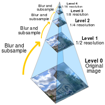
Before being put into the Convolutional Neural Network (CNN) the image is first passed through a Laplacian (which is just the derivative of the Gaussian) image processing pyramid to acquire different scale maps. There were three different scale outputs of the image created, in a similar manner shown in the picture below
Network Architecture
A typical three layer (convolution of kernel with feature map, non-linearity, pooling) CNN architecture was used. The function tanh served as the non-linearity. The kernel being used were 7x7 Toeplitz matrices (matrices with constant values along their diagonals). The pooling operation was performed by the 2x2 max-pool operator.
The same network was applied to all three different sized images. Since the parameters were shared between the networks, the same connection weights were applied to all of the images, thus allowing for the detection of scale-invariant features.
For training, stochastic gradient descent was used. To avoid over-fitting, jitter, horizontal flipping, rotations between +8 and -8, and rescaling between 90 and 110% was used.
Post-Processing
Unlike previous approaches, the emphasis of this scene-labelling method was to rely on a highly accurate pixel labelling system. So, despite the fact that a variety of approaches were attempted, including SuperPixels, Conditional Random Fields and gPb, the simple approach of super-pixels often yielded state of the art results.
