nonparametric Latent Feature Models for Link Prediction

Introduction

The goal of this paper <ref>Kurt T. Miller, Thomas L. Griffiths, and Michael I. Jordan. Nonparametric latent feature models for link prediction. NIPS, 2009</ref>is link prediction for a partially observed network, i.e. we observe the links (1 or 0) between some pairs of the nodes in a network and we try to predict the unobserved links. Basically, it builds the model by extracting the latent structure that representing the properties of individual entities. Unlike the latent space model <ref>Peter D. Hoff, Adrian E. Raftery, and Mark S. Handcock. Latent space approaches to social network analysis. JASA, 97(460):1090-1098.</ref>, which tries to find the location (arbitrary real valued features) of each node in a latent space, the "latent feature" here mainly refers to a class-based (binary features) representation. They assume a finite number of classes that entities can belong to and the interactions between classes determine the structure of the network. More specifically, the probability of forming a link depends only on the classes of the corresponding pair of nodes. The idea is fairly similar to the stochastic blockmodel <ref>Krzysztof Nowicki and Tom A. B. Snijders. Estimation and prediction for stochastic blockstructures. JASA, 96(455):1077-1087, 2001. </ref> <ref>Edoardo M. Airoldi, David M. Blei, Eric P. Xing, and Stephen E. Fienberg. Mixed membership stochastic block models. In Advances in Neural Information Processing Systems. 2009.</ref>. However, the blockmodels are mainly for community detection/network clustering, but not link prediction. This paper fills in the gap.

The nonparametric latent feature relational model is a Bayesian nonparametric model in which each node has binary-valued latent features that influences its relation to other nodes. Known covariates information can also be incorporated. The model can simultaneously infer the number (dimension) of latent features, the values of the features for each node and how the features influence the links.

The nonparametric latent feature relational model

Directed network is considered here. Let [math]\displaystyle{ Y }[/math] be the [math]\displaystyle{ N\times N }[/math] binary adjacency matrix of a network. The component [math]\displaystyle{ y_{ij}=1 }[/math] if there is a link from node [math]\displaystyle{ i }[/math] to node [math]\displaystyle{ j }[/math] and [math]\displaystyle{ y_{ij}=0 }[/math] if there is no link. The components corresponding to unobserved links are left unfilled. The goal is to learn from the observed links so that we can predict the unfilled entries.

Basic model

Let [math]\displaystyle{ Z }[/math] denote the latent features, where [math]\displaystyle{ Z }[/math] is a [math]\displaystyle{ N\times K }[/math] binary matrix. Each row of [math]\displaystyle{ Z }[/math] corresponds to a node and each column correspond to a latent feature such that [math]\displaystyle{ z_{ij}=1 }[/math] if the [math]\displaystyle{ i^{th} }[/math] node has feature [math]\displaystyle{ k }[/math] and 0, otherwise. And let [math]\displaystyle{ Z_i }[/math] denote the [math]\displaystyle{ i^{th} }[/math] row of [math]\displaystyle{ Z }[/math] (the feature vector corresponding to node i). Let W be a [math]\displaystyle{ K\times K }[/math] real-valued weight matrix where [math]\displaystyle{ w_{kk^\prime} }[/math] is the weight that affects the probability of a link when the corresponding nodes have features [math]\displaystyle{ k }[/math] and [math]\displaystyle{ k^' }[/math], respectively. By assuming the link probabilities are conditional independent give the latent features and the weights, the likelihood function can be written as:

[math]\displaystyle{ Pr(Y|Z, W)=\prod_{i,j}Pr(y_{ij}|Z_i,Z_j, W):=\sigma(Z_i W Z_j^{\top})=\sigma(\sum_{k,k^'}z_{ik}z_{jk^'}w_{kk^'}) }[/math]

where [math]\displaystyle{ \sigma(.) }[/math] is a function that transforms values from [math]\displaystyle{ (-\infty,\infty) }[/math] to [math]\displaystyle{ (0,1) }[/math].

Prior distributions are assumed for the latent features and the weight matrix, where Z is generated by Indian Buffet Process <ref>Thomas L. Griffiths and Zoubin Ghahramani. Infinite latent feature models and the Indian Buffet Process. In Advances in Neural Information Processing Systems, 2007</ref> and the component of W has normal prior, i.e.

[math]\displaystyle{ Z \sim IBP(\alpha) }[/math]

[math]\displaystyle{ w_{kk^'}\sim \mathcal{N}(0, \sigma_w^2) }[/math]

Full model

The covariates information of each node can be incorporate into the model. The full nonparametric latent feature relational model is

[math]\displaystyle{ Pr(y_{ij}=1|Z, W, X, \beta, a, b, c)=\sigma(Z_i W Z_j^\top +\beta^\top X_{ij}+(\beta_p^\top X_{p,i}+a_i)+(\beta_c^\top X_{c,i}+b_i)+c) }[/math]

where [math]\displaystyle{ X_{p,i},X_{c,j} }[/math] are known covariate vector when node i and j are link parent and child, respectively; [math]\displaystyle{ X_{ij} }[/math] is a vector of interaction effects; [math]\displaystyle{ \beta, \beta_p, \beta_c, a and b }[/math] are coefficients and offsets which all assumed to be normally distributed. We drop the corresponding terms if no information available.

Generalizations

The model can be easily generalized for multiple relations instead of a single relation. The latent features keep the same, but an independent weight matrix [math]\displaystyle{ W^i }[/math] is used for each relation [math]\displaystyle{ Y^i }[/math]. Covariates may be relation specific or common across all relations. By taking the weight matrix to be symmetric, the model can deal with undirected networks.

Inference

Exact inference for the proposed nonparametric latent feature model is infeasible. The authors adopt Markov Chain Monte Carlo (MCMC) for approximate inference (posterior inference on Z and W). They alternatively sample from Z and W. During the procedure, the all zero Z columns are dropped, since they do not provide any information.

1. Given W, resample Z

Since the IBP is exchangeable, so when sample the [math]\displaystyle{ i^{th} }[/math] row of Z, they assume that the [math]\displaystyle{ i^{th} }[/math] customer is the last one in the process. Let [math]\displaystyle{ m_k }[/math] denote the number of non-zero entries in column k, the component [math]\displaystyle{ z_{ik} }[/math] is sampled by

[math]\displaystyle{ Pr(z_{ik}=1|Z_{-ik},W,Y) \propto m_k Pr(Y|z_{ik}=1,Z_{-ik},W) }[/math]

Regarding the number of features, they use the fact that in the IBP, the prior distribution on the number of new features for the last customer is [math]\displaystyle{ Poisson(\alpha/N) }[/math]. They mentioned that the number of new features should be weighted by the corresponding likelihood term.

2. Given Z, reample W

They sequentially resample each of the weights in W that correspond to non-zero features and drop the ones corresponding to the all-zero features. The difficulty is that we do not have a conjugate prior on W, so direct resampling W from its posterior is infeasible. Some auxiliary sampling trick and MCMC procedures are used.

3. Other issues

Conjugate priors may be placed on the hyperparameters as well. In the case of multiple relations, one can sample W_i given Z independently for each i. In the full model, the posterior updates for the coefficients and intercepts are independent.

Another important issue is that the IBP often mix slowly due the large state space full of local optima. The key is to choose a good initialization.

Simulations and real data results

Synthetic data

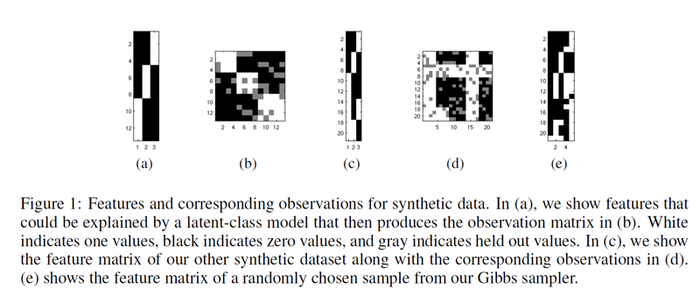
The basic model is applied to simple synthetic datasets generated from known features (shown in Figure 1(a), (c)). W is initialized randomly. The basic model is able to attain 100% accuracy on held-out data. However, it reveals the problem that the model is not able to address the latent features. This is due to subtle interactions (confounding) between sets of features and weights. So the feature inferred will not in general correspond to interpretable features. It also indicates that there are local optima in the feature space, which means a good initialization is necessary.

Multi-relational datasets

In this session, the NLFM is applied to several datasets from the Infinite Relational Model(IRM) paper <ref>Charles Kemp, Joshua B. Tenenbaum, Thomas L. Griffiths, Takeshi Yamada, and Naonori Ueda. Learning systems of concepts with an infinite relational model. In Proceedings of the American Association for Artificial Intelligence (AAAI), 2006.</ref>. One dataset contains 54 relations of 14 countries along with 90 given features of the countries. Another dataset contains 26 kinship relationships of 104 people in the Alyawarra tribe in Central Australia. The model is compared to two other class-based algorithms, the IRM and the MMSB (Mixed Membership Stochastic Blockmodel).

For each dataset, 80% of the data are used as training set and the AUC (area under the ROC curve) is reported for the held-out data (the 20% left data). Note that the closer the AUC to 1, the better. For the latent feature relational model, either a random feature matrix or class-based features from the IRM is used as initializations. The following table shows the results. It can be seen the LFRM out-performs both the IRM and MMSB.

Predicting NIPS coauthorship

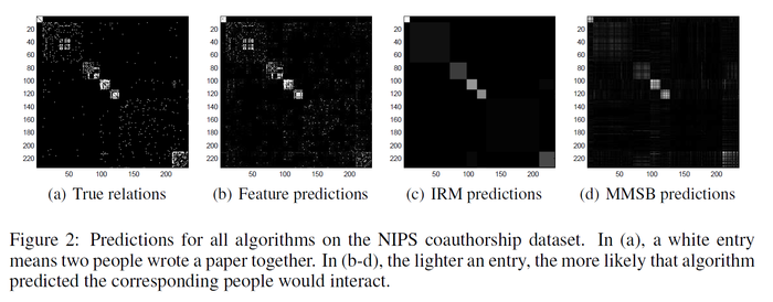
LFRM is applied to the NIPS dataset, which contains a list of all papers and authors from NIPS 1-17. The 234 authors who published with the most other people are investigated. Again, 80% data is used as training set and the rest 20% is test set. The figure below clearly shows that LFRM performs better than IMR and MMSB. The AUC values are LFRM w/IRM 0.9509 > LFRM rand 0.9466 > IRM 0.8906 > MMSB 0.8705.

Conclusion

In this paper, a nonparametric latent feature relational model is proposed for inferring latent binary features in relational entities, and link prediction. The model combines the ideas of latent feature modeling in networks with Bayesian nonparametrics inference. It can infer the dimension of feature space simultaneously when inferring the entities of the features. The model performs better than established class-based models, e.g. IRM and MMSB. The reason is that the NLFM is richer and more complex.

Discussion

1. The model sets up a new framework for network modeling.

2. It performs well in terms of estimating and predicting.

3. However, the algorithm is quite complicated and unsophisticated.

4. The algorithm highly depends on the initial values, which means one need to run another algorithm, e.g. IRM, for initial value.

5. The inferred latent features are not interpretable due to the confounding with the weight matrix.

References

<references/>