stat340s13

Introduction, Class 1 - Tuesday, May 7

{{

 Template:namespace detect

| type = style | image = | imageright = | style = | textstyle = | text = This article may require cleanup to meet Wikicoursenote's quality standards. The specific problem is: use math environment and LaTex notations for formulas. For example instead of y=1-e^(-λx) write [math]\displaystyle{ y=1-e^{-\lambda x} }[/math]. Please improve this article if you can. | small = | smallimage = | smallimageright = | smalltext = }}

Course Instructor: Ali Ghodsi

Lecture:
001: TTh 8:30-9:50 MC1085
002: TTh 1:00-2:20 DC1351
Tutorial:
2:30-3:20 Mon M3 1006

Midterm

Monday June 17 2013 from 2:30-3:30

TA(s):

TA	Day	Time	Location
Lu Cheng	Monday	3:30-5:30 pm	M3 3108, space 2
Han ShengSun	Tuesday	4:00-6:00 pm	M3 3108, space 2
Yizhou Fang	Wednesday	1:00-3:00 pm	M3 3108, space 1
Huan Cheng	Thursday	3:00-5:00 pm	M3 3111, space 1
Wu Lin	Friday	11:00-1:00 pm	M3 3108, space 1

Four Fundamental Problems

1. Classification: Given an input object X, we have a function which will take in this input X and identify which 'class (Y)' it belongs to (Discrete Case)

  i.e taking value from x, we could predict y.

(For example, an image of a fruit can be classified, through some sort of algorithm to be a picture of either an apple or an orange.)
2. Regression: Same as classification but in the continuous case except y is discrete
3. Clustering: Use common features of objects in same class or group to form clusters.(in this case, x is given, y is unknown)
4. Dimensionality Reduction (aka Feature extraction, Manifold learning)

Applications

Most useful when structure of the task is not well understood but can be characterized by a dataset with strong statistical regularity
Examples:

• Computer Vision, Computer Graphics, Finance (fraud detection), Machine Learning
  
• Search and recommendation (eg. Google, Amazon)
  
• Automatic speech recognition, speaker verification
  
• Text parsing
  
• Face identification
  
• Tracking objects in video
  
• Financial prediction(e.g. credit cards)
  
• Fraud detection
  
• Medical diagnosis
  

Course Information

Prerequisite: (One of CS 116, 126/124, 134, 136, 138, 145, SYDE 221/322) and (STAT 230 with a grade of at least 60% or STAT 240) and (STAT 231 or 241)

Antirequisite: CM 361/STAT 341, CS 437, 457

General Information

• No required textbook
• Recommended: "Simulation" by Sheldon M. Ross
• Computing parts of the course will be done in Matlab, but prior knowledge of Matlab is not essential (will have a tutorial on it)
• First midterm will be held on Monday, June 17 from 2:30 to 3:30
• Announcements and assignments will be posted on Learn.
• Other course material on: http://wikicoursenote.com/wiki/
• Log on to both Learn and wikicoursenote frequently.
• Email all questions and concerns to UWStat340@gmail.com. Do not use your personal email address!

Wikicourse note (10% of final mark): When applying an account in the wikicourse note, please use the quest account as your login name while the uwaterloo email as the registered email. This is important as the quest id will use to identify the students who make the contributions. Example:
User: questid
Email: questid@uwaterloo.ca
After the student has made the account request, do wait for several hours before students can login into the account using the passwords stated in the email. During the first login, students will be ask to create a new password for their account.

As a technical/editorial contributor: Make contributions within 1 week and do not copy the notes on the blackboard.

Must do both All contributions are now considered general contributions you must contribute to 50% of lectures for full marks

• A general contribution can be correctional (fixing mistakes) or technical (expanding content, adding examples, etc) but at least half of your contributions should be technical for full marks

Do not submit copyrighted work without permission, cite original sources. Each time you make a contribution, check mark the table. Marks are calculated on honour system, although there will be random verifications. If you are caught claiming to contribute but didn't, you will lose marks.

Wikicoursenote contribution form : [1]

- you can submit your contributions in multiple times.
- you will be able to edit the response right after submitting
- send email to make changes to an old response : uwstat340@gmail.com

Tentative Topics

- Random variable and stochastic process generation
- Discrete-Event Systems
- Variance reduction
- Markov Chain Monte Carlo

Tentative Marking Scheme

Item	Value
Assignments (~6)	30%
WikiCourseNote	10%
Midterm	20%
Final	40%

The final exam is going to be closed book and only non-programmable calculators are allowed A passing mark must be achieved in the final to pass the course

Sampling (Generating random numbers), Class 2 - Thursday, May 9

Introduction

Some people believe that sampling activities such as rolling a dice and flipping a coin are not truly random but are deterministic, since the result can be reliably calculated using things such as physics and math. In general, a deterministic model produces specific results given certain inputs by the model user, contrasting with a stochastic model which encapsulates randomness and probabilistic events.

A computer cannot generate truly random numbers because computers can only run algorithms, which are deterministic in nature. They can, however, generate Pseudo Random Numbers; numbers that seem random but are actually deterministic. Although the pseudo random numbers are deterministic, these numbers have a sequence of value and all of them have the appearances of being independent uniform random variables. Being deterministic, pseudo random numbers are valuable and beneficial due to the ease to generate and manipulate.

Mod

Let [math]\displaystyle{ n \in \N }[/math] and [math]\displaystyle{ m \in \N^+ }[/math], then by Division Algorithm, [math]\displaystyle{ \exists q, \, r \in \N \;\text{with}\; 0\leq r \lt m, \; \text{s.t.}\; n = mq+r }[/math], where [math]\displaystyle{ q }[/math] is called the quotient and [math]\displaystyle{ r }[/math] the remainder. Hence we can define a binary function [math]\displaystyle{ \mod : \N \times \N^+ \rightarrow \N }[/math] given by [math]\displaystyle{ r:=n \mod m }[/math] which means take the remainder after division by m.

We say that n is congruent to r mod m if n = mq + r, where m is an integer.

For example:
30 = 4 * 7 + 2 mod 7
30 = 2 mod 7

Note: [math]\displaystyle{ \mod }[/math] here is different from the modulo congruence relation in [math]\displaystyle{ \Z_m }[/math], which is an equivalence relation instead of a function.

Multiplicative Congruential Algorithm

This is a simple algorithm used to generate uniform pseudo random numbers. It is also referred to as the Linear Congruential Method or Mixed Congruential Method. We define the Linear Congruential Method to be [math]\displaystyle{ x_{k+1}=(ax_k + b) \mod m }[/math], where [math]\displaystyle{ x_k, a, b, m \in \N, \;\text{with}\; a, m \gt 0 }[/math]. ( [math]\displaystyle{ \mod m }[/math] means taking the remainder after division by m) Given a "seed"(all integers and an initial value x0 called seed) [math]\displaystyle{ .(x_0 \in \N }[/math], we can obtain values for [math]\displaystyle{ x_1, \, x_2, \, \cdots, x_n }[/math] inductively. The Multiplicative Congruential Method may also refer to the special case where [math]\displaystyle{ b=0 }[/math].

An interesting fact about Linear Congruential Method is that it is one of the oldest and best-known pseudorandom number generator algorithms. It is very fast and requires minimal memory to retain state. However, this method should not be used for applications where high-quality randomness is required. They should not be used for Monte Carlo simulation and cryptographic applications.

First consider the following algorithm
[math]\displaystyle{ x_{k+1}=x_{k} \mod m }[/math]

Example
[math]\displaystyle{ \text{Let }x_{0}=10,\,m=3 }[/math]

[math]\displaystyle{ \begin{align} x_{1} &{}= 10 &{}\mod{3} = 1 \\ x_{2} &{}= 1 &{}\mod{3} = 1 \\ x_{3} &{}= 1 &{}\mod{3} =1 \\ \end{align} }[/math]

[math]\displaystyle{ \ldots }[/math]

Excluding x0, this example generates a series of ones. In general, excluding x0, the algorithm above will always generate a series of the same number less than m. Hence, it has a period of 1. We can modify this algorithm to form the Multiplicative Congruential Algorithm.

Multiplicative Congruential Algorithm
[math]\displaystyle{ x_{k+1}=(a \cdot x_{k} + b) \mod m }[/math]

Example
[math]\displaystyle{ \text{Let }a=2,\, b=1, \, m=3, \, x_{0} = 10 }[/math]
[math]\displaystyle{ \begin{align} \text{Step 1: } 0&{}=(2\cdot 10 + 1) &{}\mod 3 \\ \text{Step 2: } 1&{}=(2\cdot 0 + 1) &{}\mod 3 \\ \text{Step 3: } 0&{}=(2\cdot 1 + 1) &{}\mod 3 \\ \end{align} }[/math]
[math]\displaystyle{ \ldots }[/math]

This example generates a sequence with a repeating cycle of two integers.

(If we choose the numbers properly, we could get a sequence of "random" numbers. However, how do we find the value of [math]\displaystyle{ a,b, }[/math] and [math]\displaystyle{ m }[/math]? At the very least [math]\displaystyle{ m }[/math] should be a very large, preferably prime number. The larger [math]\displaystyle{ m }[/math] is, the higher possibility people get a sequence of "random" numbers. This is easier to solve in Matlab. In Matlab, the command rand() generates random numbers which are uniformly distributed in the interval (0,1)). Matlab uses [math]\displaystyle{ a=7^5, b=0, m=2^{31}-1 }[/math] – recommended in a 1988 paper, "Random Number Generators: Good Ones Are Hard To Find" by Stephen K. Park and Keith W. Miller (Important part is that [math]\displaystyle{ m }[/math] should be large and prime)

MatLab Instruction for Multiplicative Congruential Algorithm:
Before you start, you need to clear all existing defined variables and operations:

>>clear all
>>close all

>>a=17
>>b=3
>>m=31
>>x=5
>>mod(a*x+b,m)
ans=26
>>x=mod(a*x+b,m)

(Note:
1. Keep repeating this command over and over again and you will seem to get random numbers – this is how the command rand works in a computer.
2. There is a function in MATLAB called RAND to generate a number between 0 and 1.
3. If we would like to generate 1000 and more numbers, we could use a for loop)

(Note on MATLAB commands:
1. clear all: clears all variables.
2. close all: closes all figures.
3. who: displays all defined variables.
4. clc: clears screen.)

>>a=13
>>b=0
>>m=31
>>x(1)=1
>>for ii=2:1000
x(ii)=mod(a*x(ii-1)+b,m);
end
>>size(x)
ans=1    1000
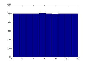
>>hist(x)

(Note: The semicolon after the x(ii)=mod(a*x(ii-1)+b,m) ensures that Matlab will not print the entire vector of x. It will instead calculate it internally and you will be able to work with it. Adding the semicolon to the end of this line reduces the run time significantly.)

This algorithm involves three integer parameters [math]\displaystyle{ a, b, }[/math] and [math]\displaystyle{ m }[/math] and an initial value, [math]\displaystyle{ x_0 }[/math] called the seed. A sequence of numbers is defined by [math]\displaystyle{ x_{k+1} = ax_k+ b \mod m }[/math]. [math]\displaystyle{ \mod m }[/math] means taking the remainder after division by [math]\displaystyle{ m }[/math].

Note: For some bad [math]\displaystyle{ a }[/math] and [math]\displaystyle{ b }[/math], the histogram may not looks uniformly distributed.

Note: hist(x) will generate a graph about the distribution. Use it after run the code to check the real sample distribution.

Example: [math]\displaystyle{ a=13, b=0, m=31 }[/math]
The first 30 numbers in the sequence are a permutation of integers from 1 to 30, and then the sequence repeats itself so it is important to choose [math]\displaystyle{ m }[/math] large to decrease the probability of each number repeating itself too early. Values are between [math]\displaystyle{ 0 }[/math] and [math]\displaystyle{ m-1 }[/math]. If the values are normalized by dividing by [math]\displaystyle{ m-1 }[/math], then the results are approximately numbers uniformly distributed in the interval [0,1]. There is only a finite number of values (30 possible values in this case). In MATLAB, you can use function "hist(x)" to see if it looks uniformly distributed.

If [math]\displaystyle{ x_0=1 }[/math], then

[math]\displaystyle{ x_{k+1} = 13x_{k}\mod{31} }[/math]

So,

[math]\displaystyle{ \begin{align} x_{0} &{}= 1 \\ x_{1} &{}= 13 \times 1 + 0 &{}\mod{31} = 13 \\ x_{2} &{}= 13 \times 13 + 0 &{}\mod{31} = 14 \\ x_{3} &{}= 13 \times 14 + 0 &{}\mod{31} =27 \\ \end{align} }[/math]

etc.

For example, with [math]\displaystyle{ a = 3, b = 2, m = 4, x_0 = 1 }[/math], we have:

[math]\displaystyle{ x_{k+1} = (3x_{k} + 2)\mod{4} }[/math]

So,

[math]\displaystyle{ \begin{align} x_{0} &{}= 1 \\ x_{1} &{}= 3 \times 1 + 2 \mod{4} = 1 \\ x_{2} &{}= 3 \times 1 + 2 \mod{4} = 1 \\ \end{align} }[/math]

etc.

---

FAQ:

1.Why in the example above is 1 to 30 not 0 to 30?
[math]\displaystyle{ b = 0 }[/math] so in order to have [math]\displaystyle{ x_k }[/math] equal to 0, [math]\displaystyle{ x_{k-1} }[/math] must be 0 (since [math]\displaystyle{ a=13 }[/math] is relatively prime to 31). However, the seed is 1. Hence, we will never observe 0 in the sequence.
Alternatively, {0} and {1,2,...,30} are two orbits of the left multiplication by 13 in the group [math]\displaystyle{ \Z_{31} }[/math].
2.Will the number 31 ever appear?Is there a probability that a number never appears?
The number 31 will never appear. When you perform the operation [math]\displaystyle{ \mod m }[/math], the largest possible answer that you could receive is [math]\displaystyle{ m-1 }[/math]. Whether or not a particular number in the range from 0 to [math]\displaystyle{ m - 1 }[/math] appears in the above algorithm will be dependent on the values chosen for [math]\displaystyle{ a, b }[/math] and [math]\displaystyle{ m }[/math].

---

Examples:[From Textbook]
If [math]\displaystyle{ x_0=3 }[/math] and [math]\displaystyle{ x_n=(5x_{n-1}+7)\mod 200 }[/math], find [math]\displaystyle{ x_1,\cdots,x_{10} }[/math].
Solution:
[math]\displaystyle{ \begin{align} x_1 &{}= (5 \times 3+7) &{}\mod{200} &{}= 22 \\ x_2 &{}= 117 &{}\mod{200} &{}= 117 \\ x_3 &{}= 592 &{}\mod{200} &{}= 192 \\ x_4 &{}= 2967 &{}\mod{200} &{}= 167 \\ x_5 &{}= 14842 &{}\mod{200} &{}= 42 \\ x_6 &{}= 74217 &{}\mod{200} &{}= 17 \\ x_7 &{}= 371092 &{}\mod{200} &{}= 92 \\ x_8 &{}= 1855467 &{}\mod{200} &{}= 67 \\ x_9 &{}= 9277342 &{}\mod{200} &{}= 142 \\ x_{10} &{}= 46386717 &{}\mod{200} &{}= 117 \\ \end{align} }[/math]

Comments:
Typically, it is good to choose [math]\displaystyle{ m }[/math] such that [math]\displaystyle{ m }[/math] is large, and [math]\displaystyle{ m }[/math] is prime. Careful selection of parameters '[math]\displaystyle{ a }[/math]' and '[math]\displaystyle{ b }[/math]' also helps generate relatively "random" output values, where it is harder to identify patterns. For example, when we used a composite (non prime) number such as 40 for [math]\displaystyle{ m }[/math], our results were not satisfactory in producing an output resembling a uniform distribution.

The computed values are between 0 and [math]\displaystyle{ m-1 }[/math]. If the values are normalized by dividing by [math]\displaystyle{ m-1 }[/math], their result is numbers uniformly distributed on the interval [math]\displaystyle{ \left[0,1\right] }[/math] (similar to computing from uniform distribution).

From the example shown above, if we want to create a large group of random numbers, it is better to have large [math]\displaystyle{ m }[/math] so that the random values generated will not repeat after several iterations.

There has been a research about how to choose uniform sequence. Many programs give you the options to choose the seed. Sometimes the seed is chosen by CPU.

Inverse Transform Method

This method is useful for generating types of distribution other than uniform distribution, such as exponential distribution and normal distribution. However, to easily use this method in generating pseudorandom numbers, the probability distribution consumed must have a cumulative distribution function (cdf) [math]\displaystyle{ F }[/math] with a tractable inverse [math]\displaystyle{ F^{-1} }[/math].

Theorem:
If U ~ U[0,1] then the random variable [math]\displaystyle{ x=F^{-1}(U) }[/math] has the distribution function F(•)
Where [math]\displaystyle{ F(x) = P(X }[/math] ≤ [math]\displaystyle{ x) }[/math] is the CDF and;
[math]\displaystyle{ F^{-1}(U) }[/math]denotes the inverse function of F(•) Or that [math]\displaystyle{ F(x)=U }[/math] [math]\displaystyle{ \Rightarrow }[/math] [math]\displaystyle{ x=F^{-1}(U) }[/math]

Proof of the theorem:
For all u є [0,1] and for all x є [math]\displaystyle{ F^{-1}(U) }[/math], the generalized inverse satisfies F([math]\displaystyle{ F^{-1}(u) }[/math]) > u and [math]\displaystyle{ F^{-1}(F(x)) }[/math] < x, Therefore,

[math]\displaystyle{ F(x) = P(X }[/math] ≤ [math]\displaystyle{ x) }[/math]
[math]\displaystyle{ = P(F^{-1}(U) }[/math] ≤ [math]\displaystyle{ x) }[/math]
[math]\displaystyle{ = P(F(F^{-1}(U)) }[/math] ≤ [math]\displaystyle{ F(x)) }[/math]  ::"Since f(x)<f(y) for x<=y"
[math]\displaystyle{ = P(U }[/math] ≤ [math]\displaystyle{ F(x)) }[/math] ::"Since F^{-1}(F(x))=x, if F is invertible"
[math]\displaystyle{ = F(x) }[/math]  ::"Because [math]\displaystyle{ Pr(U }[/math] ≤ [math]\displaystyle{ y)=y }[/math],since U is uniform on the unit interval"

Therefore, in order to generate a random variable X~F, it can generate U according to U(0,1) and then make the transformation x=[math]\displaystyle{ F^{-1}(U) }[/math]

Note that we can apply the inverse on both sides in the proof of the inverse transform only if the pdf of X is monotonic. A monotonic function is one that is either increasing for all x, or decreasing for all x.

Example: [math]\displaystyle{ f(x) = \lambda e^{-\lambda x} }[/math]
[math]\displaystyle{ F(x)= \int_0^x f(x) dx }[/math]
[math]\displaystyle{ = \int_0^x \lambda e ^{-\lambda x}\ dx }[/math]
[math]\displaystyle{ = \frac{\lambda}{-\lambda}\, e^{-\lambda x}\, | \underset{0}{x} }[/math]
[math]\displaystyle{ = -e^{\lambda x} + e^0 }[/math]
[math]\displaystyle{ =1 - e^{- \lambda x} }[/math]
[math]\displaystyle{ y=1-e^{- \lambda x} }[/math]
[math]\displaystyle{ 1-y=e^{- \lambda x} }[/math]
[math]\displaystyle{ x=-ln(1-y)/{\lambda} }[/math]
[math]\displaystyle{ y=-ln(1-x)/{\lambda} }[/math]
[math]\displaystyle{ F^{-1}(x)=-ln(1-x)/{\lambda} }[/math]

Step 1: Draw U ~U[0,1];
Step 2: [math]\displaystyle{ x=\frac{-ln(1-U)}{\lambda} }[/math]

Example: [math]\displaystyle{ X= a + (b-a), }[/math] U is uniform on [a, b]
[math]\displaystyle{ x=\frac{-ln(U)}{\lambda} }[/math] is exponential with parameter [math]\displaystyle{ {\lambda} }[/math]

Example 2: Given a CDF of X: [math]\displaystyle{ F(x) = x^5 }[/math], transform U~U[0,1].
Sol: Let [math]\displaystyle{ y=x^5 }[/math], solve for x: [math]\displaystyle{ x=y^{1/5} }[/math]. Therefore, [math]\displaystyle{ F^{-1} (x) = x^{1/5} }[/math]
Hence, to obtain a value of x from F(x), we first set u as an uniform distribution, then obtain the inverse function of F(x), and set [math]\displaystyle{ x= u^{1/5} }[/math]

Example 3: Given u~U[0,1], generate x from BETA(1,β)
Solution:
F(x)= 1-(1-x)^β
u= 1-(1-x)^β
Solve for x:
(1-x)^β = 1-u
1-x = (1-u)^(1/β)
x = 1-(1-u)^(1/β)

Example 4-Estimating pi: Let's use rand() and Monte Carlo Method to estimate [math]\displaystyle{ pi }[/math]
N= total number of points
Nc = total number of points inside the circle
Prob[(x,y) lies in the circle]=[math]\displaystyle{ Area of circle/Area of Square }[/math]
If we take square of size 2, circle will have area pi.
Thus pi= [math]\displaystyle{ 4*(Nc/N) }[/math]

Matlab Code:

N=10000;Nc=0;a=0,b=2; for t=1:1000
x=a+(b-a)*rand()
y=a+(b-a)*rand()</math>
if (x-1).^2+(y-1).^2<=1
Nc=Nc+1;
end
end

In Matlab, you can use functions: "who" to see what variables you have defined "clear all" to clear all variables you have defined "close all" to close all figures

MatLab for Inverse Transform Method:

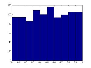
>>u=rand(1,1000)
>>hist(u)       #will generate a fairly uniform diagram

#let λ=2 in this example; however, you can make another value for λ
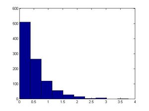
>>x=(-log(1-u))/2;
>>size(x)       #1000 in size 
>>figure
>>hist(x)       #exponential 

Limitations:
1. This method is flawed since not all functions are invertible nor monotonic.
2. It may be impractical since some CDF's and/or integrals are not easy to compute such as Gaussian distribution.

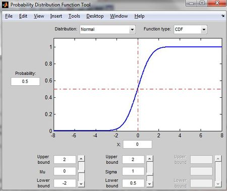
Probability Distribution Function Tool in MATLAB

>>disttool         #shows different distributions

This command allows users to explore the effect of changes of parameters on the plot of either a CDF or PDF.

(Generating random numbers continue) Class 3 - Tuesday, May 14

Recall the Inverse Transform Method

1. Draw U~U(0,1)
2. X = F^-1(U)

Proof
First note that [math]\displaystyle{ P(U\leq a)=a, \forall a\in[0,1] }[/math]

[math]\displaystyle{ P(X\leq x) }[/math]

[math]\displaystyle{ = P(F^{-1}(U)\leq x) }[/math]
[math]\displaystyle{ = P((F(F^{-1}(U))\leq F(x)) }[/math] (since [math]\displaystyle{ F(\cdot ) }[/math] is monotonically increasing)
[math]\displaystyle{ = P(U\leq F(x)) }[/math]
[math]\displaystyle{ = F(x) }[/math]

This is the c.d.f. of X.

Note: that the CDF of a U(a,b) random variable is:

[math]\displaystyle{ F(x)= \begin{cases} 0 & \text{for }x \lt a \\[8pt] \frac{x-a}{b-a} & \text{for }a \le x \lt b \\[8pt] 1 & \text{for }x \ge b \end{cases} }[/math]

Thus, for U~U(0,1), we have [math]\displaystyle{ P(U\leq 1) = 1 }[/math] and [math]\displaystyle{ P(U\leq 1/2) = 1/2 }[/math].
More generally, we see that [math]\displaystyle{ P(U\leq a) = a }[/math].
For this reason, we had [math]\displaystyle{ P(U\leq F(x)) = F(x) }[/math].

Reminder:
This is only for uniform distribution [math]\displaystyle{ U~ \sim~ Unif [0,1] }[/math]
[math]\displaystyle{ P (U \le 1) = 1 }[/math]
[math]\displaystyle{ P (U \le 0.5) = 0.5 }[/math]

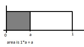[math]\displaystyle{ P(U\lt =a)=a }[/math]

LIMITATIONS OF THE INVERSE TRANSFORM METHOD

Though this method is very easy to use and apply it does have disadvantages/limitations:

1. We have to find the inverse c.d.f function F^-1(.) in some cases this does not exist

2. For many distributions such as Gaussian, it is too difficult to find the inverse cdf function , making this method inefficient

Discrete Case

We want to generate a discrete random variable x, that has probability mass function: In general in the discrete case, we have [math]\displaystyle{ x_0, \dots , x_n }[/math] where:

[math]\displaystyle{ \begin{align}P(X = x_i) &{}= p_i \end{align} }[/math]

[math]\displaystyle{ x_0 \leq x_1 \leq x_2 \dots \leq x_n }[/math]

[math]\displaystyle{ \sum p_i = 1 }[/math]

Algorithm for applying Inverse Transformation Method in Discrete Case:
1: Draw [math]\displaystyle{ U~ \sim~ Unif [0,1] }[/math]
2. [math]\displaystyle{ X=x_i, }[/math] if [math]\displaystyle{ F(x_{i-1})\lt U\leq F(x_i) }[/math]

Example in class: (Coin Flipping Example)
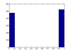
We want to simulate a coin flip. We have U~U(0,1) and X = 0 or X = 1.

We can define the U function so that:

If U <= 0.5, then X = 0

and if 0.5 < U <= 1, then X =1.

This allows the probability of Heads occurring to be 0.5 and is a good generator of a random coin flip.

[math]\displaystyle{ U~ \sim~ Unif [0,1] }[/math]

[math]\displaystyle{ \begin{align} P(X = 0) &{}= 0.5\\ P(X = 1) &{}= 0.5\\ \end{align} }[/math]

• Notice: For the bounds of X, it does not matter where you place the "=" sign; since U is a continuous random variable, the probability of f(x) equal to a point is zero.

• Code
  

>>for ii=1:1000
    u=rand;
      if u<0.5
         x(ii)=0;
      else
         x(ii)=1;
      end
  end
>>hist(x)

Note: The role of semi-colon in Matlab: Matlab will not print out the results if the line ends in a semi-colon and vice versa.

Example in class:

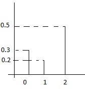
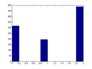
Suppose we have the following discrete distribution:

[math]\displaystyle{ \begin{align} P(X = 0) &{}= 0.3 \\ P(X = 1) &{}= 0.2 \\ P(X = 2) &{}= 0.5 \end{align} }[/math]

The cumulative density function (cdf) for this distribution is then:

[math]\displaystyle{ F(x) = \begin{cases} 0, & \text{if } x \lt 0 \\ 0.3, & \text{if } x \lt 1 \\ 0.5, & \text{if } x \lt 2 \\ 1, & \text{if } x \gt 2 \end{cases} }[/math]

Then we can generate numbers from this distribution like this, given [math]\displaystyle{ U \sim~ Unif[0, 1] }[/math]:

[math]\displaystyle{ x = \begin{cases} 0, & \text{if } U\leq 0.3 \\ 1, & \text{if } 0.3 \lt U \leq 0.5 \\ 2, & \text{if } 0.5 \lt U\leq 1 \end{cases} }[/math]

• Code (as shown in class)
  

Use Editor window to edit the code

>>close all
>>clear all
>>for ii=1:1000
    u=rand;
       if u<0.3
          x(ii)=0;
       elseif u<0.5
          x(ii)=1;
       else
          x(ii)=2;
       end
    end
>>size(x)
>>hist(x)

Example: Generating a Bernoulli random variable

[math]\displaystyle{ \begin{align} P(X = 1) = p, P(X = 0) = 1 - p\end{align} }[/math]

[math]\displaystyle{ F(x) = \begin{cases} 1-p, & \text{if } x \lt 1 \\ 1, & \text{if } 1 \leq x \end{cases} }[/math]

1. Draw [math]\displaystyle{ U~ \sim~ Unif [0,1] }[/math]
2. [math]\displaystyle{ X = \begin{cases} 1, & \text{if } U\leq p \\ 0, & \text{if } U \gt p \end{cases} }[/math]

Example: Generating Geometric Distribution:

Consider Geo(p) where p is the probability of success, and define random variable X such that X is the number of failure before the first success. x=1,2,3..... We have pmf: [math]\displaystyle{ P(X=x_i) = p*(1-p)^{x_{i-1}} }[/math] We have CDF: [math]\displaystyle{ F(x)=P(X \leq x)=1-P(X\gt x) = 1-(1-p)^x }[/math], P(X>x) means we get at least x failures before observe the first success. Now consider the inverse transform:

[math]\displaystyle{ x = \begin{cases} 1, & \text{if } U\leq p \\ 2, & \text{if } p \lt U \leq 1-(1-p)^2 \\ 3, & \text{if } 1-(1-p)^2 \lt U\leq 1-(1-p)^3 \\ .... k, & \text{if } 1-(1-p)^{k-1} \lt U\leq 1-(1-p)^k .... \end{cases} }[/math]

Note: Unlike the continuous case, the discrete inverse-transform method can always be used for any discrete distribution (but it may not be the most efficient approach)

General Procedure
1. Draw U ~ U(0,1)
2. If [math]\displaystyle{ U \leq P_{0} }[/math] deliver [math]\displaystyle{ x = x_{0} }[/math]
3. Else if [math]\displaystyle{ U \leq P_{0} + P_{1} }[/math] deliver [math]\displaystyle{ x = x_{1} }[/math]
4. Else if [math]\displaystyle{ U \leq P_{0} + P_{1} + P_{2} }[/math] deliver [math]\displaystyle{ x = x_{2} }[/math]
...

  Else if [math]\displaystyle{ U \leq P_{0} + ... + P_{k}  }[/math] deliver [math]\displaystyle{ x = x_{k} }[/math]

The problem with the inverse transformation method is that we have to find [math]\displaystyle{ F^{-1} }[/math] while not all functions have an inverse. Unfortunately, with many distributions such as the Gaussian(also known as Normal distribution, the only difference is Gaussian is represented by standard deviation while normal is represented by variance) , it is too difficult to find the inverse of [math]\displaystyle{ F(x) }[/math]. In this case, another alternative is to use the acceptance-rejection method that follows.

Acceptance-Rejection Method

Although the inverse transformation method does allow us to change our uniform distribution, it has two limits;

1. Not all functions have inverse functions (ie, the range of x and y have limit and do not fix the inverse functions)
2. For some distributions, such as Gaussian, it is too difficult to find the inverse

To generate random samples for these functions, we will use different methods, such as the Acceptance-Rejection Method.

Suppose we want to draw random sample from a target density function f(x), x∈S_x, where S_x is the support of f(x). If we can find some constant c(≥1) and a density function g(x) having the same support S_x so that f(x)≤cg(x), ∀x∈S_x, then we can apply the procedure for Acceptance-Rejection Method. Typically we choose a density function that we already know how to sample from for g(x).

{{

 Template:namespace detect

| type = style | image = | imageright = | style = | textstyle = | text = This article may require cleanup to meet Wikicoursenote's quality standards. The specific problem is: Do not write [math]\displaystyle{ c*g(x) }[/math]. Instead write [math]\displaystyle{ c \times g(x) }[/math] or [math]\displaystyle{ \,c g(x) }[/math]. Please improve this article if you can. | small = | smallimage = | smallimageright = | smalltext = }}

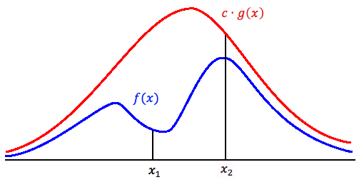
Note: If the red line was only g(x) as opposed to [math]\displaystyle{ \,c g(x) }[/math] (i.e. c=1), then [math]\displaystyle{ g(x) \geq f(x) }[/math] for all values of x iff g and f are the same functions. This is because both g(x) and f(x) are pdfs, so the area under each function is equal to 1.
To elaborate further on this, notice that g(x) is larger than f(x) for the entire visible domain. However, if we observe the tails over a large enough domain, we will notice that after some point f will become larger than g. This happens because we are looking at pdfs, as mentioned above.

Also remember that [math]\displaystyle{ \,c g(x) }[/math] always generates higher probability than what we need. Thus we need an approach of getting the proper probabilities.

c must be chosen so that [math]\displaystyle{ f(x)\eqslantless \,c g(x) }[/math] for all value of x. c can only equal 1 when f and g have the same distribution. Otherwise:
Either use a software package to test if [math]\displaystyle{ f(x)\eqslantless \, c g(x) }[/math] for an arbitrarily chosen c > 0, or:
1. Find first and second derivatives of f(x) and g(x).
2. Identify and classify all local and absolute maximums and minimums, using the First and Second Derivative Tests, as well as all inflection points.
3. Verify that [math]\displaystyle{ f(x)\eqslantless \, c g(x) }[/math] at all the local maximums as well as the absolute maximums.
4. Verify that [math]\displaystyle{ f(x)\eqslantless \, c g(x) }[/math] at the tail ends by calculating [math]\displaystyle{ \lim_{x \to +\infty} \frac{f(x)}{\, c g(x)} }[/math] and [math]\displaystyle{ \lim_{x \to -\infty} \frac{f(x)}{\, c g(x)} }[/math] and seeing that they are both < 1. Use of L'Hopital's Rule should make this easy, since both f and g are p.d.f's, resulting in both of them approaching 0.

c should be close to 1, otherwise there is a high chance we will end up rejecting our sample.

value around x₁ will be sampled more often under cg(x) than under f(x).<=More samples than we actually need, if [math]\displaystyle{ \frac{f(y)}{\, c g(y)} }[/math] is small, the acceptance-rejection technique will need to be done to these points to get the accurate amount.In the region above x₁, we should accept less and reject more.

around x₂:number of sample that are drawn and the number we need are much closer. So in the region above x₂, we accept more. As a result, g(x) and f(x) are comparable.

Another way to understand why the the acceptance probability is [math]\displaystyle{ \frac{f(y)}{\, c g(y)} }[/math], is by thinking of areas. From the graph above, we see that the target function in under the proposed function c g(y). Therefore, [math]\displaystyle{ \frac{f(y)}{\, c g(y)} }[/math] is the proportion or the area under c g(y) that also contains f(y). Therefore we say we accept sample points for which u is less then [math]\displaystyle{ \frac{f(y)}{\, c g(y)} }[/math] because then the sample points are guaranteed to fall under the area of c g(y) that contains f(y).

Procedure

1. Draw Y~g(.)
2. Draw U~u(0,1) (Note: U and Y are independent)
3. If [math]\displaystyle{ u\leq \frac{f(y)}{cg(y)} }[/math] (which is [math]\displaystyle{ P(accepted|y) }[/math]) then x=y, else return to Step 1
   

Note: Recall [math]\displaystyle{ P(U\leq a)=a }[/math]. Thus by comparing u and [math]\displaystyle{ \frac{f(y)}{\, c g(y)} }[/math], we can get a probability of accepting y at these points. For instance, at some points that cg(x) is much larger than f(x), the probability of accepting x=y is quite small.
ie. At X₁, low probability to accept the point since f(x) much smaller than cg(x).
At X₂, high probability to accept the point. [math]\displaystyle{ P(U\leq a)=a }[/math] in Uniform Distribution.

Note: Since U is the variable for uniform distribution between 0 and 1. It equals to 1 for all. The condition depends on the constant c. so the condition changes to [math]\displaystyle{ c\leq \frac{f(y)}{g(y)} }[/math]

Proof

We want to show that P(x)(which is original distribution) can be obtained/sampled using a known distribution g(y). Therefore, mathematically we want to show that:
[math]\displaystyle{ P(x) = P(y|accepted) = f(y) }[/math]

[math]\displaystyle{ P(y|accepted)=f(y) }[/math]

[math]\displaystyle{ P(y|accepted)=\frac{P(accepted|y)P(y)}{P(accepted)} }[/math]

Recall the conditional probability formulas:

[math]\displaystyle{ P(a|b)=\frac{P(a,b)}{P(b)} }[/math], or [math]\displaystyle{ P(a|b)=\frac{P(b|a)P(a)}{P(b)} }[/math]

based on the concept from procedure-step1:
[math]\displaystyle{ P(y)=g(y) }[/math]

[math]\displaystyle{ P(accepted|y)=\frac{f(y)}{cg(y)} }[/math]
(the higher the value is the larger the chance it will be selected)

[math]\displaystyle{ \begin{align} P(accepted)&=\int_y\ P(accepted|y)P(y)\\ &=\int_y\ \frac{f(s)}{cg(s)}g(s)ds\\ &=\frac{1}{c} \int_y\ f(s) ds\\ &=\frac{1}{c} \end{align} }[/math]

Therefore:
[math]\displaystyle{ \begin{align} P(x)&=P(y|accepted)\\ &=\frac{\frac{f(y)}{cg(y)}g(y)}{1/c}\\ &=\frac{\frac{f(y)}{c}}{1/c}\\ &=f(y)\end{align} }[/math]

Here is an alternative introduction of Acceptance-Rejection Method

Comments:

-Acceptance-Rejection Method is not good for all cases. One obvious cons is that it could be very hard to pick the g(y) and the constant c in some cases. And usually, c should be a small number otherwise the amount of work when applying the method could be HUGE.
-Note: When f(y) is very different than g(y), it is less likely that the point will be accepted as the ratio above would be very small and it will be difficult for u to be less than this small value.

Acceptance-Rejection Method
Example 1 (discrete case)
We wish to generate X~Bi(2,0.5), assuming that we cannot generate this directly.
We use a discrete distribution DU[0,2] to approximate this.
f(x)=Pr(X=x)=2Cx*(0.5)^2

x	0	1	2
f(x)	1/4	1/2	1/4
g(x)	1/3	1/3	1/3
c=f(x)/g(x)	3/4	3/2	3/4
f(x)/(c*g(x))	1/2	1	1/2

Since we need c>=f(x)/g(x)
We need c=3/2

Therefore, the algorithm is:
1. Generate u,v~U(0,1)
2. Set y=floor(3*u) (This is using uniform distribution to generate DU[0,2]
3. If (y=0) and (v<1/2), output=0
If (y=2) and (v<1/2), output=2
Else if y=1, output=1

An elaboration of “c”
c is the expected number of times the code runs to output 1 random variable. Remember that when u < f(x)/(c*g(x)) is not satisfied, we need to go over the code again.

Proof

Let f(x) be the function we wish to generate from, but we cannot use inverse transform method to generate directly.
Let g(x) be the helper function
Let kg(x)>=f(x)
Since we need to generate y from g(x),
Pr(select y)=g(y)
Pr(output y|selected y)=Pr(u<f(y)/(c*g(y)))= (y)/(c*g(y)) (Since u~Unif(0,1))
Pr(output y)=Pr(output y1|selected y1)Pr(select y1)+ Pr(output y2|selected y2)Pr(select y2)+…+ Pr(output yn|selected yn)Pr(select yn)=1/c
Consider that we are asking for expected time for the first success, it is a geometric distribution with probability of success=c
Therefore, E(X)=1/(1/c))=c

Acknowledgements: Some materials have been borrowed from notes from Stat340 in Winter 2013.

Example of Acceptance-Rejection Method

Generating a random variable having p.d.f.

                               [math]\displaystyle{ f(x) = 20x(1 - x)^3,         0\lt  x \lt 1   }[/math]  

Since this random variable (which is beta with parameters 2, 4) is concentrated in the interval (0, 1), let us consider the acceptance-rejection method with

                                    g(x) = 1,           0 < x < 1

To determine the constant c such that f(x)/g(x) <= c, we use calculus to determine the maximum value of

                                   f(x)/g(x) = 20x(1 - x)^3

Differentiation of this quantity yields

                                  [math]\displaystyle{ d/dx[f(x)/g(x)]=20*[(1-x)^3-3x(1-x)^2] }[/math]

Setting this equal to 0 shows that the maximal value is attained when x = 1/4, and thus,

                                 [math]\displaystyle{ f(x)/g(x)\lt = 20*(1/4)*(3/4)^3=135/64=c  }[/math]                                   

Hence,

                                 [math]\displaystyle{ f(x)/c*g(x)=(256/27)*(x*(1-x)^3) }[/math]                             

and thus the simulation procedure is as follows:

1) Generate two random numbers U1 and U2 .

2) If U₂<(256/27)*U₁*(1-U₁)³, set X=U₂, and stop Otherwise return to step 1). The average number of times that step 1) will be performed is c = 135/64.

(The above example is from http://www.cs.bgu.ac.il/~mps042/acceptance.htm, example 2.)

Simple Example of Acceptance-Rejection Method

Consider the random variable X, with distribution [math]\displaystyle{ X }[/math] ~ [math]\displaystyle{ U[0,0.5] }[/math]

So we let [math]\displaystyle{ f(x) = 2x }[/math] on [math]\displaystyle{ [0, 1/2] }[/math]

Let [math]\displaystyle{ g(.) }[/math] be [math]\displaystyle{ U[0,1] }[/math] distributed. So [math]\displaystyle{ g(x) = x }[/math] on [math]\displaystyle{ [0,1] }[/math]

Then take [math]\displaystyle{ c = 2 }[/math]

So [math]\displaystyle{ f(x)/cg(x) = (2x) / {(2)(x) } = 1 }[/math] on the interval [math]\displaystyle{ [0, 1/2] }[/math] and

[math]\displaystyle{ f(x)/cg(x) = (0) / {(2)(x) } = 0 }[/math] on the interval [math]\displaystyle{ (1/2, 1] }[/math]

So we reject:

None of the numbers generated in the interval [math]\displaystyle{ [0, 1/2] }[/math]

All of the numbers generated in the interval [math]\displaystyle{ (1/2, 1] }[/math]

And this results in the distribution [math]\displaystyle{ f(.) }[/math] which is [math]\displaystyle{ U[0,1/2] }[/math]

Another Example of Acceptance-Rejection Method

Generate a random variable from:

  [math]\displaystyle{ f(x)=3*x^2 }[/math], 0< x <1

Assume g(x) to be uniform over interval (0,1), where 0< x <1
Therefore:

  [math]\displaystyle{ c = max(f(x)/(c*g(x)))= 3 }[/math]

  [math]\displaystyle{ f(x)/(c*g(x))= x^2 }[/math]

Acknowledgement: this is example 1 from http://www.cs.bgu.ac.il/~mps042/acceptance.htm

Class 4 - Thursday, May 16

• When we want to find a target distribution, denoted as [math]\displaystyle{ f(x) }[/math]; we need to first find a proposal distribution [math]\displaystyle{ g(x) }[/math] which is easy to form.
  
• The relationship between the proposal distribution and target distribution is: [math]\displaystyle{ c \cdot g(x) \geq f(x) }[/math].
  
• Chance of acceptance is less if the distance between [math]\displaystyle{ f(x) }[/math] and [math]\displaystyle{ c \cdot g(x) }[/math] is big, and vice-versa, [math]\displaystyle{ c }[/math] keeps [math]\displaystyle{ \frac {f(x)}{c \cdot g(x)} }[/math] below 1 (so [math]\displaystyle{ f(x) \leq c*g(x) }[/math]), and we must to choose the constant [math]\displaystyle{ C }[/math] to achieve this.
  
• In other words, [math]\displaystyle{ C }[/math] is chosen to make sure [math]\displaystyle{ c \cdot g(x) \geq f(x) }[/math]. However, it will not make sense if [math]\displaystyle{ C }[/math] is simply chosen to be arbitrarily large. We need to choose [math]\displaystyle{ C }[/math] such that [math]\displaystyle{ c \cdot g(x) }[/math] fits [math]\displaystyle{ f(x) }[/math] as tightly as possible.
  

How to find C:
[math]\displaystyle{ \begin{align} &c*g(x) \geq f(x)\\ &c\geq \frac{f(x)}{g(x)} \\ &c= \max \left(\frac{f(x)}{g(x)}\right) \end{align} }[/math]

• The logic behind this:

The Acceptance-Rejection method is about to find a distribution that is known how to sample (g(x)) from and multiply by a constant c so that c*g(x) is always greater or equal to f(x). Mathematically, we want cg(x)>=f(x). And it means c has to be greater or equal to f(x)/g(x). So the smallest possible c that satisfies the condition is the maximum value of f(x)/g(x)

• For this method to be efficient, the constant c must be selected so that the rejection rate is low.
  
• It is easy to show that the expected number of trials for an acceptance is c. Thus, the smaller c is, the lower the rejection rate, and the better the algorithm:
  

Let [math]\displaystyle{ X }[/math] be the number of trials for an acceptance, [math]\displaystyle{ X \sim~ Geo(\frac{1}{c}) }[/math]

[math]\displaystyle{ \mathbb{E}[X] = \frac{1}{\frac{1}{c}} = c }[/math]

• So far, the only distribution we know how to sample from is the UNIFORM distribution.
  

Procedure:
1. Choose [math]\displaystyle{ g(x) }[/math] (simple density function that we know how to sample, i.e. Uniform so far)
The easiest case is UNIF(0,1). However, in other cases we need to generate UNIF(a,b). We may need to perform a linear transformation on the UNIF(0,1) variable.
2. Find a constant c such that :[math]\displaystyle{ c \cdot g(x) \geq f(x) }[/math]

Recall the general procedure of Acceptance-Rejection Method

1. Let [math]\displaystyle{ Y \sim~ g(y) }[/math]
2. Let [math]\displaystyle{ U \sim~ Unif [0,1] }[/math]
3. If [math]\displaystyle{ U \leq \frac{f(x)}{c \cdot g(x)} }[/math] then X=Y; else return to step 1 (This is not the way to find C. This is the general procedure.)

---

Example:Generate a random variable from the pdf

[math]\displaystyle{ f(x) = \begin{cases} 2x, & \mbox{if }0 \leqslant x \leqslant 1 \\ 0, & \mbox{otherwise} \end{cases} }[/math]

We can note that this is a special case of Beta(2,1), where, [math]\displaystyle{ beta(a,b)=\frac{\Gamma(a+b)}{\Gamma(a)\Gamma(b)}x^{(a-1)}(1-x)^{(b-1)} }[/math]

Where Γ (n)=(n-1)! if n is positive integer

Aside: Beta function In mathematics, the beta function, also called the Euler integral of the first kind, is a special function defined by [math]\displaystyle{ B(x,y)=\int_0^1 \! {t^(x-1)}{(1-t)^(y-1)}\,dt }[/math]

[math]\displaystyle{ beta(2,1)= \frac{\Gamma(3)}{(\Gamma(2)\Gamma(1))}x^1 (1-x)^0 = 2x }[/math]

---

[math]\displaystyle{ g~u(0,1) }[/math]
[math]\displaystyle{ y~g }[/math]
[math]\displaystyle{ f(x)\lt =(c(g(x)) }[/math]
[math]\displaystyle{ c\gt =\frac{f(x)}{g(x)} }[/math]
[math]\displaystyle{ c = max \frac{f(x)}{g(x)} }[/math]
we assume g is uniform. g~u(0,1)
[math]\displaystyle{ c = max (2x/1), 0\lt =x\lt =1 }[/math]
Taking x = 1 gives the highest possible c, which is c=2
Note that c is a scalar greater than 1.

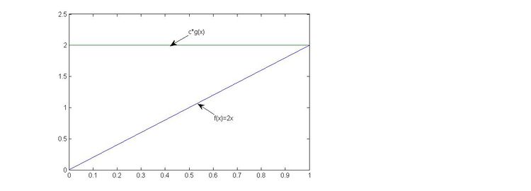
Note: g follows uniform distribution, it only covers half of the graph which runs from 0 to 1 on y-axis. Thus we need to multiply by c to ensure that c*g can cover entire f(x) area. In this case, c=2, so that makes g runs from 0 to 2 on y-axis which covers f(x).

Comment: From the picture above, we could observe that the area under f(x)=2x is a half of the area under the pdf of UNIF(0,1). This is why in order to sample 1000 points of f(x) we need to sample approximately 2000 points in UNIF(0,1). And in general, if we want to sample n points from a distritubion with pdf f(x), we need to scan approximately n*c points from the proposal distribution (g(x)) in total.
Step

1. Draw y~u(0,1)
2. Draw u~u(0,1)
3. if u<=(2*y)/(2*1), x=y
   else go to 1

Matlab Code

close all
clear all
ii=1;
jj=1;
while ii<1000
  y=rand;
  u=rand;
  jj=jj+1;
  if u<=Y
    x(ii)=y;
    ii=ii+1;
  end
end

*Note: The reason that a for loop is not used is that we need continue the looping until we get 1000 successful samples. We will reject some samples during the process and therefore do not know the number of y we are going to generate.

*Note2: In this example, we used c=2, which means we accept half of the points we generate on average. Generally speaking, 1/c would be the probability of acceptance, and an indicator of the efficiency of your chosen proposal distribution and algorithm.

*Note3: We use while instead of for when looping because we do not know how many iterations are required to generate 1000 successful samples.

---

Use Inverse Method for this Example

[math]\displaystyle{ F(x)=\int_0^x \! 2s\,ds={x^2} -0={x^2} }[/math]

[math]\displaystyle{ y=x^2 }[/math]

[math]\displaystyle{ x=\sqrt y }[/math]

[math]\displaystyle{ F^{-1}\left (\, x \, \right) =\sqrt x }[/math]

• Procedure

1: Draw [math]\displaystyle{ U~ \sim~ Unif [0,1] }[/math]

2: [math]\displaystyle{ x=F^{-1}\left (\, u\, \right) =\sqrt u }[/math]

Matlab Code

U=rand(1,1000)
x=U.^.5

Matlab Tip: Periods, ".", are used to describe the operation you want performed on each element of a vector. In the above example, to take the square root of every element in U, the notation U.^0.5 is used. However if you want to take the Square root of the entire matrix U the period, "*.*" would be excluded. i.e. Let matrix B=U^0.5, then [math]\displaystyle{ B^T*B=U }[/math]

Example of Acceptance-Rejection Method

[math]\displaystyle{ f(x)=3x^2, 0\lt x\lt 1; }[/math] [math]\displaystyle{ g(x)=1, 0\lt x\lt 1 }[/math]

[math]\displaystyle{ c = max \frac{f(x)}{g(x)} = max \frac{3x^2}{1} = 3 }[/math]
[math]\displaystyle{ \frac{f(x)}{c \cdot g(x)} = x^2 }[/math]

1. Generate two uniform numbers u₁ and u₂ 2. If [math]\displaystyle{ u_2 \leqslant (u_1)^2 }[/math], accept u₁ as the random variable from f, if not return to Step 1

We can also use g(x)=2x for a more efficient algorithm

[math]\displaystyle{ c = max \frac{f(x)}{g(x)} = max \frac {3x^2}{2x} = \frac {3x}{2} }[/math] Use the inverse method to sample from g(x) [math]\displaystyle{ G(x)=x^2 }[/math] Generate U from U(0,1) and set [math]\displaystyle{ x=sqrt(u) }[/math]

1. Generate two uniform numbers u₁ and u₂ 2. If [math]\displaystyle{ u_2\lt =3sqrt(u_1)/2 }[/math], accept u₁ as the random variable from f, if not return to Step 1

Possible Limitations

This method could be computationally inefficient depending on the rejection rate. We may have to sample many points before
we get the 1000 accepted points. For example in the example we did in class relating the f(x)=2x,
we had to sample around 2070 points before we finally accepted 1000 sample points.

Acceptance - Rejection Method Application on Normal Distribution

X ∼ N(μ,σ²); X = σZ + μ; Z ~ N(0,1)
|Z| has probability function of

f(x) = (2/[math]\displaystyle{ \sqrt{2\pi} }[/math]) e^-x2/2

g(x) = e^-x

Take h(x) = f(x)/g(x) and solve for h'(x) = 0 to find x so that h(x) is maximum.

Hence x=1 maximizes h(x) => c = [math]\displaystyle{ \sqrt{2e/\pi} }[/math]

Thus f(y)/cg(y) = e^-(y-1)2/2

How to transform [math]\displaystyle{ U(0,1) }[/math] to [math]\displaystyle{ U(a, b) }[/math]

1. Draw U from [math]\displaystyle{ U(0,1) }[/math]

2. Take [math]\displaystyle{ Y=(b-a)U+a }[/math]

3. Now Y follows [math]\displaystyle{ U(a,b) }[/math]

Example: Generate a random variable z from the Semicircular density [math]\displaystyle{ f(x)= \frac{2}{\pi R^2} \sqrt{R^2-x^2}, -R\leq x\leq R }[/math].

-> Proposal distribution: UNIF(-R, R)

-> We know how to generate using [math]\displaystyle{ U \sim UNIF (0,1) }[/math] Let [math]\displaystyle{ Y= 2RU-R=R(2U-1) }[/math]

Now, we need to find c: Since c=max[f(x)/g(x)], where
[math]\displaystyle{ f(x)= \frac{2}{\pi R^2} \sqrt{R^2-x^2} }[/math], [math]\displaystyle{ g(x)=\frac{1}{2R} }[/math], [math]\displaystyle{ -R\leq x\leq R }[/math]
Thus, we have to maximize R^2-x^2. => When x=0, it will be maximized. Therefore, c=4/pi. * Note: This also means that the probability of accepting a point is pi/4.

We will accept the points with limit f(x)/[c*g(x)]. Since [math]\displaystyle{ \frac{f(y)}{cg(y)}=\frac{\frac{2}{\pi R^{2}} \sqrt{R^{2}-y^{2}}}{\frac{4}{\pi} \frac{1}{2R}}=\frac{\frac{2}{\pi R^{2}} \sqrt{R^{2}-R^{2}(2U-1)^{2}}}{\frac{2}{\pi R}} }[/math]

• Note: Y= R(2U-1)

We can also get Y= R(2U-1) by using the formula y = a+(b-a)*u, to transform U~(0,1) to U~(a,b). Letting a=-R and b=R, and substituting it in the formula y = a+(b-a)*u, we get Y= R(2U-1).

Thus, [math]\displaystyle{ \frac{f(y)}{cg(y)}=\sqrt{1-(2U-1)^{2}} }[/math]

1. Draw [math]\displaystyle{ \ U }[/math] from [math]\displaystyle{ \ U(0,1) }[/math]

  [math]\displaystyle{ Y=R(2U-1) }[/math]

2. Draw [math]\displaystyle{ \ U_{1} }[/math] from [math]\displaystyle{ \ U(0,1) }[/math]

3. If [math]\displaystyle{ U_{1} \leq \sqrt{1-(2U-1)^2} x = y }[/math] else return to step 1.

The condition is [math]\displaystyle{ U_{1} \leq \sqrt{(1-(2U-1)^2)} }[/math]
[math]\displaystyle{ \ U_{1}^2 \leq 1 - (2U -1)^2 }[/math]
[math]\displaystyle{ \ U_{1}^2 - 1 \leq (2U - 1)^2 }[/math]
[math]\displaystyle{ \ 1 - U_{1}^2 \geq (2U - 1)^2 }[/math]

One more example about AR method
Let f(x)=x*e^(-x), x>0
Use g(x)=a*e^(-a*x) to generate random variable

Solution: First of all, we need to find c
c*g(x)>=f(x)
c>=f(x)/g(x)
f(x)/g(x)=x/a*exp(-(1-a)x)
take derivative with respect to x, and set it to 0 to get the maximum,
1/a*exp(-(1-a)x)-x/a*exp(-(1-a)x)*(1-a)=0
x=1/(1-a)

f(x)/g(x)=e^-1/(a*(1-a))
f(0)/g(0)=0
f(infinity)/g(infinity)=0

therefore, c= e^-1/(a*(1-a))

In order to minimize c, we need to find the appropriate a
Take derivative with respect to a and set it to be zero,
We could get a=1/2
c=4/e
Procedure:
1. Generate u v ~unif(0,1)
2. Generate y from g, since g is exponential with rate 2, let y=-ln(u)
3. If v<f(y)/(c*g(y)), output y
Else, go to 1

Acknowledgements: the example above is from notes from Stat340 in Winter 2013.