Time-series Generative Adversarial Networks
Presented By
Govind Sharma (20817244)
Introduction
A time-series model should not only be good at learning the overall distribution of temporal features within different time points, but it should also be good at capturing the dynamic relationship between the temporal variables across time.
The popular autoregressive approach in time-series or sequence analysis is generally focused on minimizing the error involved in multi-step sampling improving the temporal dynamics of data [1]. In this approach, the distribution of sequences is broken down into a product of conditional probabilities. The deterministic nature of this approach works well for forecasting but it is not very promising in a generative setup. The GAN approach when applied on time-series directly simply tries to learn [math]\displaystyle{ p(X|t) }[/math] using generator and discriminator setup but this fails to leverage the prior probabilities like in the case of the autoregressive models.
This paper proposes a novel GAN architecture that combines the two approaches (unsupervised GANs and supervised autoregressive) that allow a generative model to have the ability to preserve temporal dynamics along with learning the overall distribution. This mechanism has been termed as Time-series Generative Adversarial Network or TimeGAN. To incorporate supervised learning of data into the GAN architecture, this approach makes use of an embedding network that provides a reversible mapping between the temporal features and their latent representations. The key insight of this paper is that the embedding network is trained in parallel with the generator/discriminator network.
This approach leverages the flexibility of GANs together with the control of the autoregressive model resulting in significant improvements in the generation of realistic time-series.
Related Work
The TimeGAN mechanism combines ideas from different research threads in time-series analysis.
Due to differences between closed-loop training (ground truth conditioned) and open-loop inference (the previous guess conditioned), there can be significant prediction error in multi-step sampling in autoregressive recurrent networks [2]. Different methods have been proposed to remedy this including Scheduled Sampling [1], based on curriculum learning [2], where the models are trained to output based on a combination of ground truth and previous outputs. Another method inspired by adversarial domain adaptation is training an auxiliary discriminator that helps separate free-running and teacher-forced hidden states accelerating convergence[3][4]. Approach based on Actor-critic methods [5] have also been proposed that condition on target outputs estimating the next-token value that nudges the actor’s free-running predictions [11]. While all these proposed methods try to improve step-sampling, they are still inherently deterministic.
Direct application of GAN architecture on time-series data like C-RNN-GAN or RCGAN [6] try to generate the time-series data recurrently sometimes taking the generated output from the previous step as input (like in case of RCGAN) along with the noise vector. Recently, adding time stamp information for conditioning has also been proposed in these setups to handle inconsistent sampling. But these approaches remain very GAN-centric and depend only on the traditional adversarial feedback (fake/real) to learn which is not sufficient to capture the temporal dynamics.
Problem Formulation
Generally, time-series data can be decomposed into two components: static features (variables that remain constant over the entire time-series, or for a long period of time) and temporal features (variables that changes with respect to time). The paper uses [math]\displaystyle{ S }[/math] to denote the static component and [math]\displaystyle{ X }[/math] to denote the temporal features. Using this setting, inputs to the model can be thought of as a tuple of [math]\displaystyle{ (S, X_{1:t}) }[/math] that has a joint distribution [math]\displaystyle{ p }[/math]. The objective of a generative model is to learn from training data, an approximation of the original distribution [math]\displaystyle{ p(S, X) }[/math] i.e. [math]\displaystyle{ \hat{p}(S, X) }[/math]. Along with this joint distribution, another objective is to simultaneously learn the autoregressive decomposition of [math]\displaystyle{ p(S, X_{1:T}) = p(S)\prod_tp(X_t|S, X_{1:t-1}) }[/math] as well. This gives the following two objective functions.
Proposed Architecture
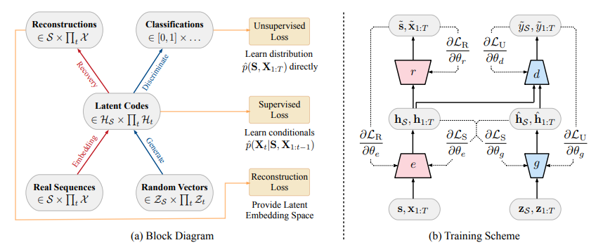
Apart from the normal GAN components of sequence generator and sequence discriminator, TimeGAN has two additional elements: an embedding function and a recovery function. As mentioned before, all these components are trained concurrently. Figure 1 shows how these four components are arranged and how the information flows between them during training in TimeGAN.
Embedding and Recovery Functions
These functions map between the temporal features and their latent representation. This mapping reduces the dimensionality of the original feature space. Let [math]\displaystyle{ H_s }[/math] and [math]\displaystyle{ H_x }[/math] denote the latent representations of [math]\displaystyle{ S }[/math] and [math]\displaystyle{ X }[/math] features in the original space. Therefore, the embedding function has the following form:
And similarly, the recovery function has the following form:
In the paper, these functions have been implemented using a recurrent network for e and a feedforward network for r. These implementation choices are of course subject to parametrization using any architecture.
Sequence Generator and Discriminator
Coming to the conventional GAN components of TimeGAN, there is a sequence generator and a sequence discriminator. But these do not work on the original space, rather the sequence generator uses the random input noise to generate sequences in the latent space. Thus, the generator takes as input the noise vectors [math]\displaystyle{ Z_s }[/math], [math]\displaystyle{ Z_x }[/math] and turns them into a latent representation [math]\displaystyle{ H_s }[/math] and [math]\displaystyle{ H_x }[/math]. This function is implemented using a recurrent network.
The discriminator takes as input the latent representation from the embedding space and produces its binary classification (synthetic/real). This is implemented using a bidirectional recurrent network with a feedforward output layer.
Architecture Workflow
The embedding and recovery functions ought to guarantee an accurate reversible mapping between the feature space and the latent space. After the embedding function turns the original data [math]\displaystyle{ (s, x_{1:t}) }[/math] into the embedding space i.e. [math]\displaystyle{ h_s }[/math], [math]\displaystyle{ h_x }[/math], the recovery function should be able to reconstruct the original data as accurately as possible from this latent representation. Denoting the reconstructed data by [math]\displaystyle{ \tilde{s} }[/math] and [math]\displaystyle{ \tilde{x}_{1:t} }[/math], we get the first objective function of the reconstruction loss:
The generator component in TimeGAN not only gets the noise vector Z as input but it also gets in autoregressive fashion, its previous output i.e. [math]\displaystyle{ h_s }[/math] and [math]\displaystyle{ h_{1:t} }[/math] as input as well. The generator uses these inputs to produce the synthetic embeddings. The unsupervised gradients when computed are used to decreasing the likelihood at the generator and increasing it at the discriminator to provide the correct classification of the produced synthetic output. This is the second objective function in the unsupervised loss form.
As mentioned before, TimeGAN does not rely on only the binary feedback from GANs adversarial component i.e. the discriminator. It also incorporates the supervised loss from the embedding and recovery functions into the fold. To ensure that the two segments of TimeGAN interact with each other, the generator is alternatively fed embeddings of actual data instead of its own previous synthetical produced embedding. Maximizing the likelihood of this produces the third objective i.e. the supervised loss:
Optimization
The embedding and recovery components of TimeGAN are trained to minimize the Supervised loss and Recovery loss. If [math]\displaystyle{ \theta_{e} }[/math] and [math]\displaystyle{ \theta_{r} }[/math] denote their parameters, then the paper proposes the following as the optimization problem for these two components:
Formula.
Here [math]\displaystyle{ \lambda }[/math] >= 0 is used to regularize (or balance) the two losses. The other components of TimeGAN i.e. generator and discriminator are trained to minimize the Supervised loss along with Unsupervised loss. This optimization problem is formulated as below:
Formula.
Here [math]\displaystyle{ \eta \gt = 0 }[/math] is used to regularize the two losses.
Experiments
In the paper, the authors compare TimeGAN with the two most familiar and related variations of traditional GANs applied to time-series i.e. RCGAN and C-RNN-GAN. To make a comparison with autoregressive approaches, the authors use RNNs trained with T-Forcing and P-Forcing. Additionally, performance comparisons are also made with WaveNet [7] and its GAN alternative WaveGAN [8]. Qualitatively, the generated data is examined in terms of diversity (healthy distribution of sample covering real data), fidelity (samples should be indistinguishable from real data), and usefulness (samples should have the same predictive purposes as real data).
The following methods are used for benchmarking and evaluation:
- Visualization: This involves the application of t-SNE and PCA analysis on data (real and synthetic). This is done to compare the distribution of generated data with the real data in 2-D space.
- Discriminative Score: This involves training a post-hoc time-series classification model (an off-the-shelf RNN) to differentiate sequences from generated and original sets.
- Predictive Score: This involves training a post-hoc sequence prediction model to forecast using the generated data and this is evaluated against the real data.
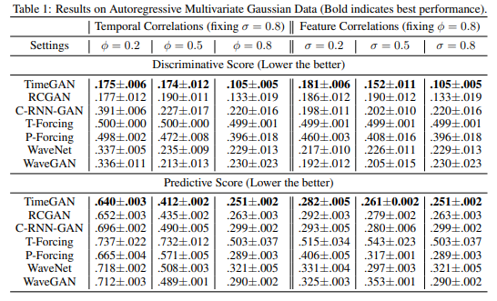
In the first experiment, the authors used time-series sequences from an autoregressive multivariate Gaussian data defined as [math]\displaystyle{ x_t=\phi x_{t-1}+n }[/math], where [math]\displaystyle{ n \sim N(0, \sigma 1 + (1-\sigma)I) }[/math]. Table 1 has the results of this experiment performed by different models. The results clearly show how TimeGAN outperforms other methods in terms of both discriminative and predictive scores.
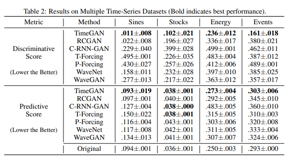
Next, the paper has experimented on different types of Time Series Data. Using time-series sequences of varying properties, the paper evaluates the performance of TimeGAN to testify for its ability to generalize over time-series data. The paper uses datasets like Sines, Stocks, Energy, and Events with different methods to see their performance.
Sines
They simulated multivariate sinusoidal sequences of different frequencies η and phases θ, providing continuous-valued, periodic, multivariate data where each feature is independent of others.
Stocks
By contrast, sequences of stock prices are continuous-valued but aperiodic; furthermore, features are correlated with each other. They use the daily historical Google stocks data from 2004 to 2019, including as features the volume and high, low, opening, closing, and adjusted closing prices.
Energy
They consider a dataset characterized by noisy periodicity, higher dimensionality, and correlated features. The UCI Appliances energy prediction dataset consists of multivariate, continuous-valued measurements including numerous temporal features measured at close intervals.
Events
Finally, they considered a dataset characterized by discrete values and irregular time stamps. They used a large private lung cancer pathways dataset consisting of sequences of events and their times, and model both the one-hot encoded sequence of event types and the event timings.
Figure 2 shows t-SNE/PCA visualization comparison for Sines and Stocks and it is clear from the figure that among all different models, TimeGAN shows the best overlap between generated and original data.
Table 2 shows a comparison of predictive and discriminative scores for different methods across different datasets. And TimeGAN outperforms other methods in both scores indicating a better quality of generated synthetic data across different types of datasets.
Source Code
The GitHub repository for the paper is https://github.com/jsyoon0823/TimeGAN .
Conclusion
Combining the flexibility of GANs and control over conditional temporal dynamics of autoregressive models, TimeGAN shows significant quantitative and qualitative gains for generated time-series data across different varieties of datasets.
The authors indicated the potential incorporation of Differential Privacy Frameworks into TimeGAN in the future in order to produce realistic time sequences with differential privacy guarantees.
Critique
The method introduced in this paper is truly a novel one. The idea of enhancing the unsupervised components of a GAN with some supervised element has shown significant jumps in certain evaluations. I think the methods of evaluation used in this paper namely, t-SNE/PCA analysis (visualization), discriminative score, and predictive score; are very appropriate for this sort of analysis where the focus is on multiple things (generative accuracy and conditional dependence) both quantitatively and qualitatively. Other related works [9] have also used the same evaluation setup.
The idea of the synthesized time-series being useful in terms of its predictive ability is good, especially in practice. But I think when the authors set out to create a model that can learn the temporal dynamics between time-series data then there could have been some additional metric that could better evaluate if the underlying temporal relations have been captured by the model or not. I feel the addition of some form of temporal correlation analysis would have added to the completeness of the paper.
The enhancement of traditional GAN by simply adding an extra loss function to the mix is quite elegant. TimeGAN uses a stepwise supervised loss. The authors have also used very common choices for the various components of the overall TimeGAN network. This leaves a lot of possibilities in this area as many direct and indirect variations of TimeGAN or other architectures inspired by TimeGAN can be developed in a very straightforward manner of hyper-parameterizing the building blocks.
TimeGAN benefits from merging supervised and unsupervised learning to create their generations while other methods in the literature benefit from learning their conditional input to create its generations. I believe after even considering the supervised and unsupervised learning, the way that the authors introduced temporal embeddings to assist network training is not designed well for anomaly detection (outlier detection) as it is only designed for time series representation learning as discussed in [10].
The paper certainly proposes a novel approach to analysing time series data, but there are concerns about the way the model is tested in practice. First, if the data is generated from a [math]\displaystyle{ VAR(1) }[/math] model, why would the authors would not use a multi-dimensional auto-ARIMA procedure, or a Box-Jenkins approach, to fit a model to their synthetic dataset. Moreover, as has been studied in the M4 competitions (see e.g. https://www.sciencedirect.com/science/article/pii/S0169207019301128), the ability of complex ML models or deep learning models to beat linear models in general is questionable. The theoretical reason for this empirical finding is that the Wold decomposition theorem says that a stationary process can be decomposed into the sum of a deterministic process and linear process, which gives a lot of credence to the ARIMA model. It would be highly beneficial if the authors included the Box-Jenkins benchmark in their experiments as well as testing their model against real data to see if it actually performs well.
References
[1] Samy Bengio, Oriol Vinyals, Navdeep Jaitly, and Noam Shazeer. Scheduled sampling for sequence prediction with recurrent neural networks. In Advances in Neural Information Processing Systems, pages 1171–1179, 2015.
[2] Yoshua Bengio, Jérôme Louradour, Ronan Collobert, and Jason Weston. Curriculum learning. In Proceedings of the 26th annual international conference on machine learning, pages 41–48. ACM, 2009.
[3] Alex M Lamb, Anirudh Goyal Alias Parth Goyal, Ying Zhang, Saizheng Zhang, Aaron C Courville, and Yoshua Bengio. Professor forcing: A new algorithm for training recurrent networks. In Advances In Neural Information Processing Systems, pages 4601–4609, 2016.
[4] Yaroslav Ganin, Evgeniya Ustinova, Hana Ajakan, Pascal Germain, Hugo Larochelle, François Laviolette, Mario Marchand, and Victor Lempitsky. Domain-adversarial training of neural networks. The Journal of Machine Learning Research, 17(1):2096–2030, 2016.
[5] Vijay R Konda and John N Tsitsiklis. Actor-critic algorithms. In Advances in neural information processing systems, pages 1008–1014, 2000.
[6] Mehdi Mirza and Simon Osindero. Conditional generative adversarial nets. arXiv preprint arXiv:1411.1784, 2014.
[7] Aäron Van Den Oord, Sander Dieleman, Heiga Zen, Karen Simonyan, Oriol Vinyals, Alex Graves, Nal Kalchbrenner, Andrew W Senior, and Koray Kavukcuoglu. Wavenet: A generative model for raw audio. SSW, 125, 2016
[8] Chris Donahue, Julian McAuley, and Miller Puckette. Adversarial audio synthesis. arXiv preprint arXiv:1802.04208, 2018
[9] Hao Ni, L. Szpruch, M. Wiese, S. Liao, Baoren Xiao. Conditional Sig-Wasserstein GANs for Time Series Generation, 2020
[10] Geiger, Alexander et al. “TadGAN: Time Series Anomaly Detection Using Generative Adversarial Networks.” ArXiv abs/2009.07769 (2020): n. pag.
[11] Dzmitry Bahdanau, Philemon Brakel, Kelvin Xu, Anirudh Goyal, Ryan Lowe, Joelle Pineau, Aaron Courville, and Yoshua Bengio. An actor-critic algorithm for sequence prediction. arXiv preprint arXiv:1607.07086, 2016.


