Semantic Relation Classification——via Convolution Neural Network

Presented by

Rui Gong, Xinqi Ling, Di Ma,Xuetong Wang

Introduction

A Semantic Relation can imply a relation between different words and a relation between different sentences or phrases. For example, the pair of words "white" and "snowy" can be synonyms, while "white" and "black" can be opposites. It can be used for recommendation systems like YouTube, and understanding sentiment analysis. The study of semantic analysis involves determining the exact meaning of a text. For example, the word "date", can have different meanings in different contexts, like a calendar "date", a "date" fruit, or a romantic "date".

One of the emerging trends of natural language technologies is their use for the humanities and sciences (Gbor et al., 2018). SemEval 2018 Task 7 mainly solves the problem of relation extraction and classification of two entities in the same sentence into 6 potential relations. The 6 relations are USAGE, RESULT, MODEL-FEATURE, PART WHOLE, TOPIC, and COMPARE.

SemEval 2018 Task 7 extracted data from 350 scientific paper abstracts, which has 1228 and 1248 annotated sentences for two tasks, respectively. For each data, an example sentence was chosen with its right and left sentences, as well as an indicator showing whether the relation is reserved, then a prediction is made.

Three models were used for the prediction: Linear Classifiers, Long Short-Term Memory(LSTM), and Convolutional Neural Networks (CNN). In the end, the prediction based on the CNN model was ultimately submitted since it performed the best among all models. By using the learned custom word embedding function, the research team added a variant of negative sampling, thereby improving performance and surpassing ordinary CNN.

Previous Work

SemEval 2010 Task 8 (Hendrickx et al., 2010) explored the classification of natural language relations and studied the 9 relations between word pairs. However, it is not designed for scientific text analysis, and their challenge differs from the challenge of this paper in its generalizability; this paper’s relations are specific to ACL papers (e.g. MODEL-FEATURE), whereas the 2010 relations are more general, and might necessitate more common-sense knowledge than the 2018 relations. Xu et al. (2015a) and Santos et al. (2015) both applied CNN with negative sampling to finish task7. The 2017 SemEval Task 10 also featured relation extraction within scientific publications.

Algorithm

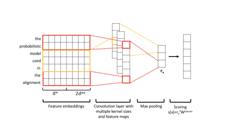
This is the architecture of CNN. We first transform a sentence via Feature embeddings. Basically, we transform each sentence into continuous word embeddings:

$$ (e^{w_i}) $$

And word position embeddings: $$ (e^{wp_i}): e_i = [e^{w_i}, e^{wp_i}] $$

In the word embeddings, we got a vocabulary ‘V’, and we will make an embedding word matrix based on the position of the word in the vocabulary. This matrix is trainable and needs to be initialized by pre-trained embedding vectors.

In the word position embeddings, we first need to input some words named ‘entities,’ and they are the key for the machine to determine the sentence’s relation. During this process, if we have two entities, we will use the relative position of them in the sentence to make the embeddings. We will output two vectors, and one of them keeps track of the first entity relative position in the sentence ( we will make the entity recorded as 0, the former word recorded as -1 and the next one 1, etc. ). And the same procedure for the second entity. Finally, we will get two vectors concatenated as the position embedding. For example, in the sentence "the black cat jumped", the position embedding of "cat" is -2,-1,0,1.

After the embeddings, the model will transform the embedded sentence into a fix-sized representation of the whole sentence via the convolution layer. Finally, after the max-pooling to reduce the dimension of the output of the layers, we will get a score for each relation class via a linear transformation.

After featurizing all words in the sentence. The sentence of length N can be expressed as a vector of length [math]\displaystyle{ N }[/math], which looks like $$e=[e_{1},e_{2},\ldots,e_{N}]$$ and each entry represents a token of the word. Also, to apply convolutional neural network, the subsets of features $$e_{i:i+j}=[e_{i},e_{i+1},\ldots,e_{i+j}]$$ are given to a weight matrix [math]\displaystyle{ W\in\mathbb{R}^{(d^{w}+2d^{wp})\times k} }[/math] to produce a new feature, defiend as $$c_{i}=\text{tanh}(W\cdot e_{i:i+k-1}+bias)$$ This process is applied to all subsets of features with length [math]\displaystyle{ k }[/math] starting from the first one. Then a mapped feature factor is produced: $$c=[c_{1},c_{2},\ldots,c_{N-k+1}]$$

The max pooling operation is used, the [math]\displaystyle{ \hat{c}=max\{c\} }[/math] was picked. With different weight filter, different mapped feature vectors can be obtained. Finally, the original sentence [math]\displaystyle{ e }[/math] can be converted into a new representation [math]\displaystyle{ r_{x} }[/math] with a fixed length. For example, if there are 5 filters, then there are 5 features ([math]\displaystyle{ \hat{c} }[/math]) picked to create [math]\displaystyle{ r_{x} }[/math] for each [math]\displaystyle{ x }[/math].

Then, the score vector $$s(x)=W^{classes}r_{x}$$ is obtained which represented the score for each class, given [math]\displaystyle{ x }[/math]'s entities' relation will be classified as the one with the highest score. The [math]\displaystyle{ W^{classes} }[/math] here is the model being trained.

To improve the performance, “Negative Sampling" was used. Given the trained data point [math]\displaystyle{ \tilde{x} }[/math], and its correct class [math]\displaystyle{ \tilde{y} }[/math]. Let [math]\displaystyle{ I=Y\setminus\{\tilde{y}\} }[/math] represent the incorrect labels for [math]\displaystyle{ x }[/math]. Basically, the distance between the correct score and the positive margin, and the negative distance (negative margin plus the second largest score) should be minimized. So the loss function is $$L=\log(1+e^{\gamma(m^{+}-s(x)_{y})})+\log(1+e^{\gamma(m^{-}-\mathtt{max}_{y'\in I}(s(x)_{y'}))})$$ with margins [math]\displaystyle{ m_{+} }[/math], [math]\displaystyle{ m_{-} }[/math], and penalty scale factor [math]\displaystyle{ \gamma }[/math]. The whole training is based on ACL anthology corpus and there are 25,938 papers with 136,772,370 tokens in total, and 49,600 of them are unique.

Results

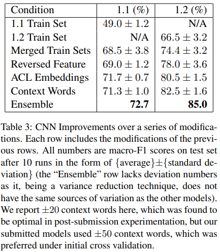
In machine learning, the most important part is to tune the hyper-parameters. Unlike traditional hyper-parameter optimization, there are some modifications to the model to increase performance on the test set. There are 5 modifications that we can apply:

1. Merged Training Sets. It combined two training sets to increase the data set size and it improves the equality between classes to get better predictions.

2. Reversal Indicate Features. It added a binary feature.

3. Custom ACL Embeddings. It embedded a word vector to an ACL-specific corps.

4. Context words. Within the sentence, it varies in size on a context window around the entity-enclosed text.

5. Ensembling. It used different early stop and random initializations to improve the predictions.

These modifications performances well on the training data and they are shown in table 3.

As we can see the best choice for this model is ensembling as the random initialization made the data more natural and avoided the overfit. During the training process, there are some methods such that they can only increase the score on the cross-validation test sets but hurt the performance on the overall macro-F1 score. Thus, these methods were eventually ruled out.

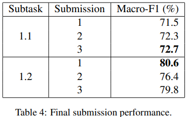
There are six submissions in total. Three for each training set and the result is shown in figure 2.

The best submission for the training set 1.1 is the third submission which does not use a separate cross-validation dataset. Instead, a constant number of training epochs are run with cross-validation based on the training data.

This compares to the other submissions in which 10% of the training data are removed to form the validation set (both with and without stratification). Predictions for these are made when the model has the highest validation accuracy.

The best submission for the training set 1.2 is the submission which extracted 10% of the training data to form the validation dataset. Predictions are made when maximum accuracy is reached on the validation data.

All in all, early stopping cannot always be based on the accuracy of the validation set since it cannot guarantee to get better performance on the real test set. Thus, we have to try new approaches and combine them to see the prediction results. Also, doing stratification will certainly improve the performance of the test data.

Conclusions

Throughout the process, we have experimented with linear classifiers, sequential random forest, LSTM, and CNN models with various variations applied, such as two models of attention, negative sampling, entity embedding or sentence-only embedding, etc.

Among all variations, vanilla CNN with negative sampling and ACL-embedding, without attention, has significantly better performance than all others. Attention-based pooling, up-sampling, and data augmentation are also tested, but they barely perform positive increment on the behavior.

Critiques

- Applying this in news apps might be beneficial to improve readability by highlighting specific important sections.

- The data set come from 350 scientist papers, this could be more explained by the author on how those paper are selected and why those paper are important to discuss.

- In the section of previous work, the author mentioned 9 natural language relationships between the word pairs. Among them, 6 potential relationships are USAGE, RESULT, MODEL-FEATURE, PART WHOLE, TOPIC, and COMPARE. It would help the readers to better understand if all 9 relationships are listed in the summary.

-This topic is interesting and this application might be helpful for some educational websites to improve their website to help readers focus on the important points. I think it will be nice to use Latex to type the equation in the sentence rather than center the equation on the next line. I think it will be interesting to discuss applying this way to other languages such as Chinese, Japanese, etc.

- It would be a good idea if the authors can provide more details regarding ACL Embeddings and Context words modifications. Scores generated using these two modifications are quite close to the highest Ensembling modification generated score, which makes it a valid consideration to examine these two modifications in detail.

- This paper is dealing with a similar problem as 'Neural Speed Reading Via Skim-RNN', num 19 paper summary. It will be an interesting approach to compare these two models' performance based on the same dataset.

- I think it would be highly practical to implement this system as a page-rank system for search engines (such as google, bing, or other platforms like Facebook, Instagram, etc.) by finding the most prevalent information available in a search query and then matching the search to the related text which can be found on webpages. This could also be implemented in search bars on specific websites or locations as well.

- It would be interesting to see in the future how the model would behave if data not already trained was used. This pre-trained data as mentioned in the paper had noise included. Using cleaner data would give better results maybe.

- The selection of the training dataset, i.e. the abstracts of scientific papers, is an excellent idea since the abstracts usually contain more information than the body. But it may be also a good idea to train the model with the conclusions. Other than that, the result of applying the model to the body part of the scientific papers may show some interesting features of the model.

-From Table4 we find that comparing with using a fixed number of training periods, early stopping based on the accuracy of the validation set does not guarantee better test set performance. The label ratio of the validation set is layered according to the training set, which helps to improve the performance of the test set. Whether it is beneficial to add entity embedding as an additional feature could be an interesting point of discussion.

References

Diederik P Kingma and Jimmy Ba. 2014. Adam: A method for stochastic optimization. arXiv preprint arXiv:1412.6980.

DragomirR. Radev, Pradeep Muthukrishnan, Vahed Qazvinian, and Amjad Abu-Jbara. 2013. The ACL anthology network corpus. Language Resources and Evaluation, pages 1–26.

Tomas Mikolov, Kai Chen, Greg Corrado, and Jeffrey Dean. 2013a. Efficient estimation of word representations in vector space. arXiv preprint arXiv:1301.3781.

Tomas Mikolov, Ilya Sutskever, Kai Chen, Greg S Corrado, and Jeff Dean. 2013b. Distributed representations of words and phrases and their compositionality. In Advances in neural information processing systems, pages 3111–3119.

Kata Gbor, Davide Buscaldi, Anne-Kathrin Schumann, Behrang QasemiZadeh, Hafa Zargayouna, and Thierry Charnois. 2018. Semeval-2018 task 7:Semantic relation extraction and classification in scientific papers. In Proceedings of the 12th International Workshop on Semantic Evaluation (SemEval2018), New Orleans, LA, USA, June 2018.