Streaming Bayesian Inference for Crowdsourced Classification
Group 4 Paper Presentation Summary
By Jonathan Chow, Nyle Dharani, Ildar Nasirov
Motivation
Crowdsourcing can be a useful tool for data generation in classification projects by collecting annotations of large groups. Typically, this takes the form of online questions which many respondents will manually answer for payment. One example of this is Amazon's Mechanical Turk, a website where businesses (or "requesters") will remotely hire individuals(known as "Turkers" or "crowdsourcers") to perform human intelligence tasks (tasks that computers cannot do). In theory, it is effective in processing high volumes of small tasks that would be expensive to achieve in other methods.
The primary limitation of this method to acquire data is that respondents can submit incorrect responses so that we couldn't ensure the data quality.
Therefore, the success of crowdsourcing is limited by how well ground-truth can be determined. The primary method for doing so is probabilistic inference. However, current methods are computationally expensive, lack theoretical guarantees, or are limited to specific settings. In the meantime, there are some approaches to focus on how we sample the data from the crowd, rather than how we aggregate it to improve the accuracy of the system.
Dawid-Skene Model for Crowdsourcing
The one-coin Dawid-Skene model is popular for contextualizing crowdsourcing problems. For task [math]\displaystyle{ i }[/math] in set [math]\displaystyle{ M }[/math], let the ground-truth be the binary [math]\displaystyle{ y_i = {\pm 1} }[/math]. We get labels [math]\displaystyle{ X = {x_{ij}} }[/math] where [math]\displaystyle{ j \in N }[/math] is the index for that worker.
We assume that we interact with workers in sequential fashion. At each time step [math]\displaystyle{ t }[/math], a worker [math]\displaystyle{ j = a(t) }[/math] provides their label for an assigned task [math]\displaystyle{ i }[/math] and provides the label [math]\displaystyle{ x_{ij} = {\pm 1} }[/math]. We denote responses up to time [math]\displaystyle{ t }[/math] via superscript.
We let [math]\displaystyle{ x_{ij} = 0 }[/math] if worker [math]\displaystyle{ j }[/math] has not completed task [math]\displaystyle{ i }[/math]. We assume that [math]\displaystyle{ P(x_{ij} = y_i) = p_j }[/math]. This implies that each worker is independent and has equal probability of correctly labelling regardless of task. In crowdsourcing the data, we must determine how workers are assigned to tasks. We introduce two methods.
Under uniform sampling, workers are allocated to tasks such that each task is completed by the same number of workers, rounded to the nearest integer, and no worker completes a task more than once. This policy is given by
Under uncertainty sampling, we assign more workers to tasks that are less certain. Assuming, we are able to estimate the posterior probability of ground-truth, we can allocate workers to the task with the lowest probability of falling into the predicted class. This policy is given by
We then need to aggregate the data. The simple method of majority voting makes predictions for a given task based on the class the most workers have assigned it, [math]\displaystyle{ \hat{y}_i = \text{sign}\{\sum_{j \in N_i} x_{ij}\} }[/math].
Streaming Bayesian Inference for Crowdsourced Classification (SBIC)
The aim of the SBIC algorithm is to estimate the posterior probability, [math]\displaystyle{ P(y, p | X^t, \theta) }[/math] where [math]\displaystyle{ X^t }[/math] are the observed responses at time [math]\displaystyle{ t }[/math] and [math]\displaystyle{ \theta }[/math] is our prior. We can then generate predictions [math]\displaystyle{ \hat{y}^t }[/math] as the marginal probability over each [math]\displaystyle{ y_i }[/math] given [math]\displaystyle{ X^t }[/math], and [math]\displaystyle{ \theta }[/math].
We factor [math]\displaystyle{ P(y, p | X^t, \theta) \approx \prod_{i \in M} \mu_i^t (y_i) \prod_{j \in N} \nu_j^t (p_j) }[/math] where [math]\displaystyle{ \mu_i^t }[/math] corresponds to each task and [math]\displaystyle{ \nu_j^t }[/math] to each worker.
We then sequentially optimize the factors [math]\displaystyle{ \mu^t }[/math] and [math]\displaystyle{ \nu^t }[/math]. We begin by assuming that the worker accuracy follows a beta distribution with parameters [math]\displaystyle{ \alpha }[/math] and [math]\displaystyle{ \beta }[/math]. Initialize the task factors [math]\displaystyle{ \mu_i^0(+1) = q }[/math] and [math]\displaystyle{ \mu_i^0(-1) = 1 – q }[/math] for all [math]\displaystyle{ i }[/math].
When a new label is observed at time [math]\displaystyle{ t }[/math], we update the [math]\displaystyle{ \nu_j^t }[/math] of worker [math]\displaystyle{ j }[/math]. We then update [math]\displaystyle{ \mu_i }[/math]. These updates are given by
where [math]\displaystyle{ \hat{p}_j^t = \frac{\sum_{i \in M_j^{t - 1}} \mu_i^{t - 1}(x_{ij}) + \alpha}{|M_j^{t - 1}| + \alpha + \beta } }[/math].
We choose our predictions to be the maximum [math]\displaystyle{ \mu_i^t(k) }[/math] for [math]\displaystyle{ k= \{-1,1\} }[/math].
Depending on our ordering of labels [math]\displaystyle{ X }[/math], we can select for different applications.
Fast SBIC
The pseudocode for Fast SBIC is shown below.

As the name implies, the goal of this algorithm is speed. To facilitate this, we leave the order of [math]\displaystyle{ X }[/math] unchanged.
We express [math]\displaystyle{ \mu_i^t }[/math] in terms of its log-odds
where [math]\displaystyle{ z_i^0 = \log(\frac{q}{1 - q}) }[/math].
The product chain then becomes a summation and removes the need to normalize each [math]\displaystyle{ \mu_i^t }[/math]. We use these log-odds to compute worker accuracy,
where [math]\displaystyle{ \sigma(z_i^{t-1}) := \frac{1}{1 + exp(-z_i^{t - 1})} = \mu_i^{t - 1}(+1) }[/math]
The final predictions are made by choosing class [math]\displaystyle{ \hat{y}_i^T = \text{sign}(z_i^T) }[/math]. We see later that Fast SBIC has similar computational speed to majority voting.
Sorted SBIC
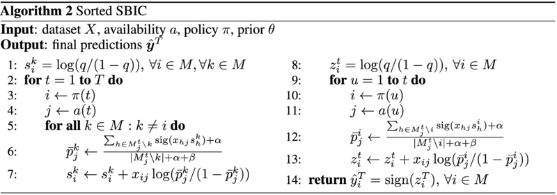
To increase the accuracy of the SBIC algorithm in exchange for computational efficiency, we run the algorithm in parallel giving labels in different orders. The pseudocode for this algorithm is given below.

From the general discussion of SBIC, we know that predictions on task [math]\displaystyle{ i }[/math] are more accurate toward the end of the collection process. This is a result of observing more data points and having run more updates on [math]\displaystyle{ \mu_i^t }[/math] and [math]\displaystyle{ \nu_j^t }[/math] to move them further from their prior. This means that task [math]\displaystyle{ i }[/math] is predicted more accurately when its corresponding labels are seen closer to the end of the process.
We take advantage of this property by maintaining a distinct “view” of the log-odds for each task. When a label is observed, we update views for all tasks except the one for which the label was observed. At the end of the collection process, we process skipped labels. When run online, this process must be repeated at every timestep.
We see that sorted SBIC is slower than Fast SBIC by a factor of M, the number of tasks. However, we can reduce the complexity by viewing [math]\displaystyle{ s^k }[/math] across different tasks in an offline setting when the whole dataset is known in advance.
Theoretical Analysis
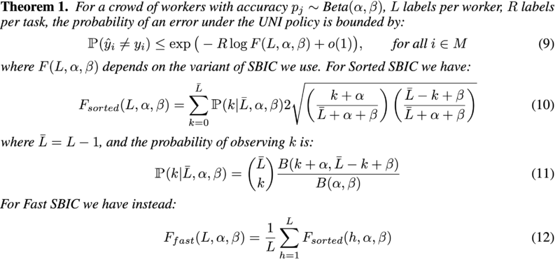
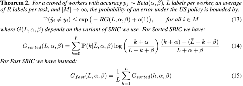
The authors prove an exponential relationship between the error probability and the number of labels per task. This allows for an upper bound to be placed on the error, in the asymptotic regime, where it can be assumed the SBIC predictions are close to the true values. The two theorems, for the different sampling regimes, are presented below.


Empirical Analysis
The purpose of the empirical analysis is to compare SBIC to the existing state of the art algorithms. The SBIC algorithm is run on five real-world binary classification datasets. The results can be found in the table below. Other algorithms in the comparison are, from left to right, majority voting, expectation-maximization, mean-field, belief-propagation, Monte-Carlo sampling, and triangular estimation.
First of all, the algorithms are run on a synthetic data that meets the assumptions of an underlying one-coin Dawid-Skene model, which allows the authors to compare SBIC's performance empirically with the theoretical results previously shown.

In bold are the best performing algorithms for each dataset. We see that both versions of the SBIC algorithm are competitive, having similar prediction errors to EM, AMF, and MC. All are considered state-of-the-art Bayesian algorithms.
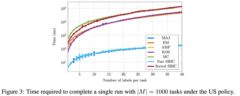
The figure below shows the average time required to simulate predictions on synthetic data under an uncertainty sampling policy. We see that Fast SBIC is comparable to majority voting and significantly faster than the other algorithms. This speed improvement, coupled with comparable accuracy, makes the Fast SBIC algorithm powerful.

Conclusion and Future Research
In conclusion, we have seen that SBIC is computationally efficient, accurate in practice, and has theoretical guarantees. The authors intend to extend the algorithm to the multi-class case in the future.
Critique
In crowdsourcing data, the cost associated with collecting additional labels is not usually prohibitively expensive. As a result, if there is concern over ground-truth, paying for additional data to ensure X is sufficiently dense may be the desired response as opposed to sacrificing ground-truth accuracy. This may result in the SBIC algorithm being less practically useful than intended. Perhaps, a study can be done to compare the cost of acquiring additional data and checking how much it improves the accuracy of ground-truth. This can help us decide the usefulness of this algorithm. Second, SBIC should be used in multiple types of data like audio, text, and images to make sure that it delivers consistent results.
The paper is tackling the classic problem of aggregating labels in a crowdsourced application, with a focus on speed. The algorithms proposed are fast and simple to implement and come with theoretical guarantees on the bounds for error rates. However, the paper starts with an objective of designing fast label aggregation algorithms for a streaming setting yet doesn’t spend any time motivating the applications in which such algorithms are needed. All the datasets used in the empirical analysis are static datasets therefore for the paper to be useful, the problem considered should be well motivated. It also appears that the output from the algorithm depends on the order in which the data is processed, which may need to be clarified. Finally, the theoretical results are presented under the assumption that the predictions of the FBI converge to the ground truth, however, the reasoning behind this assumption is not explained.
The paper assumes that crowdsourcing from human beings is systematic: that is, respondents to the problems would act in similar ways that can be classified into some categories. There are lots of other factors that need to be considered for a human respondent, such as fatigue effects and conflicts of interest. Those factors would seriously jeopardize the validity of the results and the model if they were not carefully designed and taken care of. For example, one formally accurate subject reacts badly to the subject one day generating lots of faulty data, and it would take lots of correct votes to even out the effects. Even in lots of medical experiment that involves human subjects, with rigorous standards and procedures, the results could still be invalid. The trade-off for speed while sacrificing the validity of results is not wise.
When introducing the Streaming Bayesian Inference for Crowdsourced Classification method, it was explicitly mentioned that one can select for different applications based on the ordering of labels X. However, "applications" mentioned here were not further explained or explored to support the effectiveness and meaning of developing such an algorithm. Thus, it would be sufficient for the author to build a connection between the proposed algorithm and its real-world application to make this summary more purposeful and engaging.
References
[1] Manino, Tran-Thanh, and Jennings. Streaming Bayesian Inference for Crowdsourced Classification. 33rd Conference on Neural Information Processing Systems, 2019