orthogonal gradient descent for continual learning

Authors

Mehrdad Farajtabar, Navid Azizan, Alex Mott, Ang Li

Introduction

Neural Networks suffer from catastrophic forgetting: forgetting previously learned tasks when trained to do new ones. Most neural networks can’t learn tasks sequentially despite having the capacity to learn them simultaneously. For example, training a CNN to look at only one label of CIFAR10 at a time results in poor performance for the initially trained labels (catastrophic forgetting). But that same CNN will perform really well if all the labels are trained simultaneously (as is standard). The ability to learn tasks sequentially is called continual learning, and it is crucially important for real world applications of machine learning. For example, a medical imaging classifier might be able to classify a set of base diseases very well, but its utility is limited if it cannot be adapted to learn novel diseases - like local/rare/or new diseases (like Covid-19).

This work introduces a new learning algorithm called Orthogonal Gradient Descent (OGD) that replaces Stochastic Gradient Descent (SGD). In standard SGD, the optimization takes no care to retain performance on any previously learned tasks, which works well when the task is presented all at once and iid. However, in a continual learning setting, when tasks/labels are presented sequentially, SGD fails to retain performance on earlier tasks. This is because when data is presented simultaneously, our goal is to model the underlying joint data distribution [math]\displaystyle{ P(X_1,X_2,\ldots, X_n) }[/math], and we can sample batches like [math]\displaystyle{ (X_1,X_2,\ldots, X_m) }[/math] iid from this distribution, which is assumed to be "fixed" during training. In continual learning, this distribution typically shifts over time, thus resulting in the failure of SGD. OGD considers previously learned tasks by maintaining a space of previous gradients, such that incoming gradients can be projected onto an orthogonal basis of that space - minimally impacting previously attained performance.

Previous Work

Continual learning is not a new concept in machine learning, and there are many previous research articles on the subject that can help to get acquainted with the subject ([4], [9], [10] for example). These previous works in continual learning can be summarized into three broad categories. There are expansion based techniques, which add neurons/modules to an existing model to accommodate incoming tasks while leveraging previously learned representations. One of the downsides of this method is the growing size of the model with an increasing number of tasks. There are also regularization based methods, which constraints weight updates according to some important measure for previous tasks. Finally, there are the repetition based methods. These models attempt to artificially interlace data from previous tasks into the training scheme of incoming tasks, mimicking traditional simultaneous learning. This can be done by using memory modules or generative networks.

Orthogonal Gradient Descent

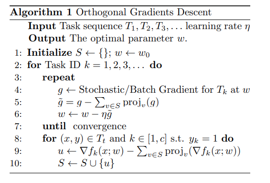
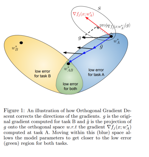
The key insight to OGD is leveraging the overparameterization of neural networks, meaning they have more parameters than data points. In order to learn new things without forgetting old ones, OGD proposes the intuitive notion of projecting newly found gradients onto an orthogonal basis for the space of previously optimal gradients. Such an orthogonal basis will exist because neural networks are typically overparameterized. Note that moving along the gradient direction results in the biggest change for parameter update, whereas moving orthogonal to the gradient results in the least change, which effectively prevents the predictions of the previous task from changing too much. A small step orthogonal to the gradient of a task should result in little change to the loss for that task, owing again to the overparameterization of the network [5, 6, 7, 8].

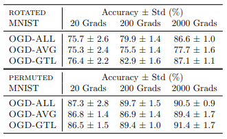
More specifically, OGD keeps track of the gradient with respect to each logit (OGD-ALL), since the idea is to project new gradients onto a space which minimally impacts the previous task across all logits. However, they have also done experiments where they only keep track of the gradient with respect to the ground truth logit (ODG-GTL) and with the logits averaged (OGD-AVE). OGD-ALL keeps track of gradients of dimension N*C where N is the size of the previous task and C is the number of classes. OGD-AVE and OGD-GTL only store gradients of dimension N since the class logits are either averaged or ignored respectively. To further manage memory, the authors sample from all the gradients of the old task, and they find that 200 is sufficient - with diminishing returns when using more.

The orthogonal basis for the span of previously attained gradients can be obtained using a simple Gram-Schmidt (or more numerically stable equivalent) iterative method. One such algorithm which can be utilized to improve numerical stability is the modified Gram-Schmidt Orthogonalisation. The issue with the simpler Gram-Schmidt algorithm can be seen in the following:

Suppose we have a matrix [math]\displaystyle{ A }[/math] which is to be decomposed into [math]\displaystyle{ A=\hat{Q}\hat{R} }[/math] using the Gram-Schmidt algorithm. During the algorithm, columns of [math]\displaystyle{ \hat{Q} }[/math] are solved sequentially, where [math]\displaystyle{ \hat{\vec{q_j}} }[/math] is the [math]\displaystyle{ j^{th} }[/math] column of [math]\displaystyle{ \hat{Q} }[/math], and [math]\displaystyle{ \hat{r_{ij}} }[/math] which is the [math]\displaystyle{ i^{th} }[/math] row and [math]\displaystyle{ j^{th} }[/math] column of [math]\displaystyle{ \hat{R} }[/math] are solved from left to right and top to bottom for only the elements [math]\displaystyle{ \hat{R} }[/math] to result in a upper triangular matrix. Consider when we are calculating the third column of [math]\displaystyle{ \hat{Q} }[/math] as follows: [math]\displaystyle{ \hat{\vec{q_{3}}}=\vec{a_3} - (\hat{\vec{q_1}}\vec{a_3})\hat{\vec{q_1}} - (\hat{\vec{q_2}}\vec{a_3})\hat{\vec{q_2}} }[/math]. [math]\displaystyle{ \vec{z_3}=\vec{a_3} - (\hat{\vec{q_1}}\vec{a_3})\hat{\vec{q_1}} }[/math] should not have a component in direction [math]\displaystyle{ \hat{\vec{q_1}} }[/math], however, due to numerical stability and catastrophic cancellation [11] this is not always true. The partial result [math]\displaystyle{ \vec{z_3} }[/math] ends up having a component in this direction, this leads to a loss in orthogonality in the columns of [math]\displaystyle{ \hat{Q} }[/math]. To remedy this problem, the modified Gram-Schmidt algorithm replaces [math]\displaystyle{ \vec{a_3} }[/math] with [math]\displaystyle{ \vec{z_3} }[/math] in [math]\displaystyle{ (\hat{\vec{q_2}}\vec{a_3})\hat{\vec{q_2}} }[/math], this helps in ensuring the orthogonality of the columns of [math]\displaystyle{ \hat{Q} }[/math] to any loss of numerical significance since we will be orthogonalizing with the vector which already has the loss of significance.

Algorithm 1 shows the precise algorithm for OGD.

And perhaps the easiest way to understand this is pictorially. Here, Task A is the previously learned task and task B is the incoming task. The neural network [math]\displaystyle{ f }[/math] has parameters [math]\displaystyle{ w }[/math] and is indexed by the [math]\displaystyle{ j }[/math]th logit.

Results

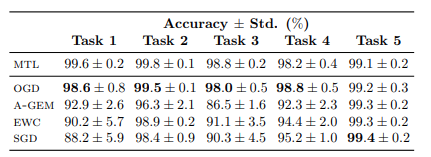
Each task was trained for 5 epochs, with tasks derived from the MNIST dataset. The network is a three-layer MLP with 100 hidden units in two layers and 10 logit outputs. The results of OGD-AVE, ODG-GTL, OGD-ALL are compared to SGD, ECW [2], (a regularization method using Fischer information for importance weights), A-GEM [3] (a state-of-the-art replay technique), and MTL (a ground truth "cheat" model which has access to all data throughout training). The experiments were performed for the following three continual learning benchmarks: permuted MNIST, rotated MNIST, and split MNIST.

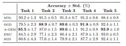
In permuted MNIST [1], there are five tasks, where each task is a fixed permutation that gets applied to each MNIST digit. The following tables show classification performance for each task after sequentially training on all the tasks. Thus, if solved catastrophic forgetting has been solved, the accuracies should be constant across tasks. If not, then there should be a significant decrease from task 5 through to task 1.

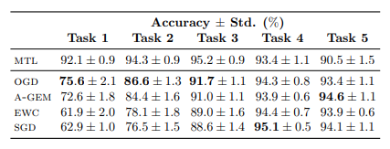
Rotated MNIST is similar except instead of fixed permutation there are fixed rotations. There are five sequential tasks, with MNIST images rotated at 0, 10, 20, 30, and 40 degrees in each task.

Split MNIST defines 5 tasks with mutually disjoint labels [4].

Also, the below table corresponds to the performance of Rotated MNIST and Permuted MNIST as a function of number of gradients stored.

Overall OGD performs much better than ECW, A-GEM, and SGD. The primary metric to look for is decreasing performance in the earlier tasks. As we can see, MTL, which represents the ideal simultaneous learning scenario shows no drop-off across tasks since all the data from previous tasks is available when training incoming tasks. For OGD, we see a decrease, but it is not nearly as severe a decrease as naively doing SGD. OGD performs much better than ECW and slightly better than A-GEM.

Review

This work presents an interesting and intuitive algorithm for continual learning. It is theoretically well-founded and shows higher performance than competing algorithms. One of the downsides is that the learning rate must be kept very small, in order to respect the assumption that orthogonal gradients do not affect the loss. Furthermore, this algorithm requires maintaining a set of gradients which grows with the number of tasks. The authors mention several directions for future study based on this technique. Finding a way to store more gradients or preauthorize the important directions can result in improved results. Secondly, all the proposed methods including this method fail when the tasks are dissimilar. Finding ways to maintain performance under tasks dissimilarity can be an interesting research direction. Thirdly, solving for learning rate sensitivity will make this method more appealing when large learning rate are desired. Finally, another interesting future work is extending the current method to other types of optimizers such as Adam and Adagrad or even second or even quasi-Newton methods.

One interesting way for increasing learning rate can be considering the gradient magnitude of the parameters for data of the former task. If for some specific parameters, the gradient magnitude for data of task A is low then intuitively it means they have not capture high amount of information from task A. Having this in mind, at least we can increase the learning rate for updating these weights so that we can use them for task B.

A valuable resource for continual learning is the following GitHub page: link continual_learning_papers

References

[1] Goodfellow, I. J., Mirza, M., Xiao, D., Courville, A., and Bengio, Y. (2013). An empirical investigation of catastrophic forgetting in gradient-based neural networks. arXiv preprint arXiv:1312.6211

[2] Kirkpatrick, J., Pascanu, R., Rabinowitz, N., Veness, J., Desjardins, G., Rusu, A. A., Milan, K., Quan, J., Ramalho, T., Grabska-Barwinska, A., et al. (2017). Overcoming catastrophic forgetting in neural networks. Proceedings of the national academy of sciences, 114(13):3521–3526.

[3] Chaudhry, A., Ranzato, M., Rohrbach, M., and Elhoseiny, M. (2018). Efficient lifelong learning with A-GEM. arXiv preprint arXiv:1812.00420.

[4] Zenke, F., Poole, B., and Ganguli, S. (2017). Continual learning through synaptic intelligence. In Proceedings of the 34th International Conference on Machine Learning-Volume 70, pages 3987–3995. JMLR

[5] Azizan, N. and Hassibi, B. (2018). Stochastic gradient/mirror descent: Minimax optimality and implicit regularization. arXiv preprint arXiv:1806.00952

[6] Li, Y. and Liang, Y. (2018). Learning overparameterized neural networks via stochastic gradient descent on structured data. In Advances in Neural Information Processing Systems, pages 8157–8166.

[7] Allen-Zhu, Z., Li, Y., and Song, Z. (2018). A convergence theory for deep learning via overparameterization. arXiv preprint arXiv:1811.03962.

[8] Azizan, N., Lale, S., and Hassibi, B. (2019). Stochastic mirror descent on overparameterized nonlinear models: Convergence, implicit regularization, and generalization. arXiv preprint arXiv:1906.03830.

[9] Nagy, D. G., & Orban, G. (2017). Episodic memory for continual model learning. ArXiv, Nips.

[10] Nguyen, C. V., Li, Y., Bui, T. D., & Turner, R. E. (2017). Variational continual learning. ArXiv, Vi, 1–18.

[11] Wikipedia: https://en.wikipedia.org/wiki/Loss_of_significance