a neural representation of sketch drawings

Introduction

In this paper, the authors present a recurrent neural network, sketch-rnn, that can be used to construct stroke-based drawings. Besides new robust training methods, they also outline a framework for conditional and unconditional sketch generation.

Neural networks have been heavily used as image generation tools. For example, Generative Adversarial Networks, Variational Inference, and Autoregressive models have been used. Most of those models are designed to generate pixels to construct images. However, people learn to draw using sequences of strokes, beginning when they are young. The authors propose a new generative model that creates vector images so that it might generalize abstract concepts in a manner more similar to how humans do.

The model is trained with hand-drawn sketches as input sequences. The model is able to produce sketches in vector format. In the conditional generation model, they also explore the latent space representation for vector images and discuss a few future applications of this model. The model and dataset are now available as an open source project (link).

Terminology

Pixel images, also referred to as raster or bitmap images are files that encode image data as a set of pixels. These are the most common image type, with extensions such as .png, .jpg, .bmp.

Vector images are files that encode image data as paths between points. SVG and EPS file types are used to store vector images.

For a visual comparison of raster and vector images, see this video. As mentioned, vector images are generally simpler and more abstract, whereas raster images generally are used to store detailed images.

For this paper, the important distinction between the two is that the encoding of images in the model will be inherently more abstract because of the vector representation. The intuition is that generating abstract representations is more effective using a vector representation.

Related Work

There are some works in the history that used a similar approach to generate images such as Portrait Drawing by Paul the Robot [26, 28] and some reinforcement learning approaches[28], Reinforcement Learning to discover a set of paint brush strokes that can best represent a given input photograph. They work more like a mimic of digitized photographs. There are also some Neural networks based approaches, but those are mostly dealing with pixel images. Little work is done on vector images generation. There are models that use Hidden Markov Models [25] or Mixture Density Networks [2] to generate human sketches, continuous data points (modelling Chinese characters as a sequence of pen stroke actions) or vectorized Kanji characters [9,29].

The model also allows us to explore the latent space representation of vector images. There are previous works that achieved similar functions as well, such as combining Sequence-to-Sequence models with Variational Autoencoder to model sentences into latent space and using probabilistic program induction to model Omniglot dataset.

The dataset they use contains 50 million vector sketches. Before this paper, there is a Sketch data with 20k vector sketches, a Sketchy dataset with 70k vector sketches along with pixel images, and a ShadowDraw system that used 30k raster images along with extracted vectorized features. They are all comparatively small.

Major Contributions

This paper makes the following major contributions: Authors outline a framework for both unconditional and conditional generation of vector images composed of a sequence of lines. The recurrent neural network-based generative model is capable of producing sketches of common objects in a vector format. The paper develops a training procedure unique to vector images to make the training more robust. The paper also made available a large dataset of hand drawn vector images to encourage further development of generative modelling for vector images, and also release an implementation of our model as an open source project

Methodology

Dataset

QuickDraw is a dataset with 50 million vector drawings collected by an online game Quick Draw!, where the players are required to draw objects belonging to a particular object class in less than 20 seconds. It contains hundreds of classes, each class has 70k training samples, 2.5k validation samples and 2.5k test samples.

The data format of each sample is a representation of a pen stroke action event. The Origin is the initial coordinate of the drawing. The sketches are points in a list. Each point consists of 5 elements [math]\displaystyle{ (\Delta x, \Delta y, p_{1}, p_{2}, p_{3}) }[/math] where x and y are the offset distance in x and y directions from the previous point. The parameters [math]\displaystyle{ p_{1}, p_{2}, p_{3} }[/math] represent three possible states in binary one-hot representation where [math]\displaystyle{ p_{1} }[/math] indicates the pen is touching the paper, [math]\displaystyle{ p_{2} }[/math] indicates the pen will be lifted from here, and [math]\displaystyle{ p_{3} }[/math] represents the drawing has ended.

Sketch-RNN

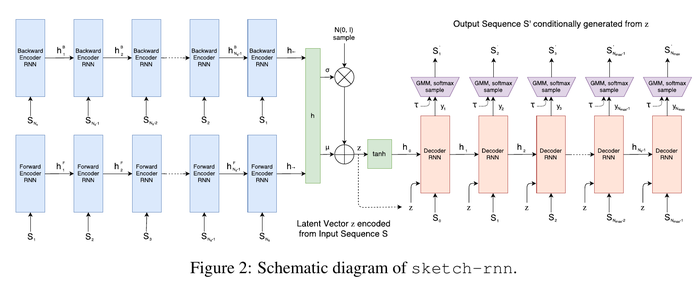
The model is a Sequence-to-Sequence Variational Autoencoder(VAE).

Encoder

The encoder is a bidirectional RNN. The input is a sketch sequence denoted by [math]\displaystyle{ S =\{S_0, S_1, ... S_{N_{s}}\} }[/math] and a reversed sketch sequence denoted by [math]\displaystyle{ S_{reverse} = \{S_{N_{s}},S_{N_{s}-1}, ... S_0\} }[/math]. The final hidden layer representations of the two encoded sequences [math]\displaystyle{ (h_{ \rightarrow}, h_{ \leftarrow}) }[/math] are concatenated to form a latent vector, [math]\displaystyle{ h }[/math], of size [math]\displaystyle{ N_{z} }[/math],

\begin{split} &h_{ \rightarrow} = encode_{ \rightarrow }(S), \\ &h_{ \leftarrow} = encode_{ \leftarrow }(S_{reverse}), \\ &h = [h_{\rightarrow}; h_{\leftarrow}]. \end{split}

Then the authors project [math]\displaystyle{ h }[/math] into two vectors [math]\displaystyle{ \mu }[/math] and [math]\displaystyle{ \hat{\sigma} }[/math] of size [math]\displaystyle{ N_{z} }[/math]. The projection is performed using a fully connected layer. These two vectors are the parameters of the latent space Gaussian distribution that will estimate the distribution of the input data. Because standard deviations cannot be negative, an exponential function is used to convert it to all positive values. Next, a random variable with mean [math]\displaystyle{ \mu }[/math] and standard deviation [math]\displaystyle{ \sigma }[/math] is constructed by scaling a normalized IID Gaussian, [math]\displaystyle{ \mathcal{N}(0,I) }[/math],

\begin{split} & \mu = W_\mu h + b_\mu, \\ & \hat \sigma = W_\sigma h + b_\sigma, \\ & \sigma = exp( \frac{\hat \sigma}{2}), \\ & z = \mu + \sigma \odot \mathcal{N}(0,I). \end{split}

Note that [math]\displaystyle{ z }[/math] is not deterministic but a random vector that can be conditioned on an input sketch sequence.

Decoder

The decoder is an autoregressive RNN. The initial hidden and cell states are generated using [math]\displaystyle{ [h_0;c_0] = \tanh(W_z z + b_z) }[/math]. Here, [math]\displaystyle{ c_0 }[/math] is utilized if applicable (eg. if an LSTM decoder is used). [math]\displaystyle{ S_0 }[/math] is defined as [math]\displaystyle{ (0,0,1,0,0) }[/math] (the pen is touching the paper at location 0, 0).

For each step [math]\displaystyle{ i }[/math] in the decoder, the input [math]\displaystyle{ x_i }[/math] is the concatenation of the previous point [math]\displaystyle{ S_{i-1} }[/math] and the latent vector [math]\displaystyle{ z }[/math]. The outputs of the RNN decoder [math]\displaystyle{ y_i }[/math] are parameters for a probability distribution that will generate the next point [math]\displaystyle{ S_i }[/math].

The authors model [math]\displaystyle{ (\Delta x,\Delta y) }[/math] as a Gaussian mixture model (GMM) with [math]\displaystyle{ M }[/math] normal distributions and model the ground truth data [math]\displaystyle{ (p_1, p_2, p_3) }[/math] as a categorical distribution [math]\displaystyle{ (q_1, q_2, q_3) }[/math] where [math]\displaystyle{ q_1, q_2\ \text{and}\ q_3 }[/math] sum up to 1,

\begin{align*} p(\Delta x, \Delta y) = \sum_{j=1}^{M} \Pi_j \mathcal{N}(\Delta x,\Delta y | \mu_{x,j}, \mu_{y,j}, \sigma_{x,j},\sigma_{y,j}, \rho _{xy,j}), where \sum_{j=1}^{M}\Pi_j = 1 \end{align*}

Where [math]\displaystyle{ \mathcal{N}(\Delta x,\Delta y | \mu_{x,j}, \mu_{y,j}, \sigma_{x,j},\sigma_{y,j}, \rho _{xy,j}) }[/math] is a bi-variate Normal Distribution, with parameters means [math]\displaystyle{ \mu_x, \mu_y }[/math], standard deviations [math]\displaystyle{ \sigma_x, \sigma_y }[/math] and correlation parameter [math]\displaystyle{ \rho_{xy} }[/math]. There are [math]\displaystyle{ M }[/math] such distributions. [math]\displaystyle{ \Pi }[/math] is a categorical distribution vector of length [math]\displaystyle{ M }[/math]. Collectively these form the mixture weights of the Gaussian Mixture model.

The output vector [math]\displaystyle{ y_i }[/math] is generated using a fully-connected forward propagation in the hidden state of the RNN.

\begin{split} &x_i = [S_{i-1}; z], \\ &[h_i; c_i] = forward(x_i,[h_{i-1}; c_{i-1}]), \\ &y_i = W_y h_i + b_y, \\ &y_i \in \mathbb{R}^{6M+3}. \\ \end{split}

The output consists the probability distribution of the next data point.

\begin{align*} [(\hat\Pi_1\ \mu_x\ \mu_y\ \hat\sigma_x\ \hat\sigma_y\ \hat\rho_{xy})_1\ (\hat\Pi_1\ \mu_x\ \mu_y\ \hat\sigma_x\ \hat\sigma_y\ \hat\rho_{xy})_2\ ...\ (\hat\Pi_1\ \mu_x\ \mu_y\ \hat\sigma_x\ \hat\sigma_y\ \hat\rho_{xy})_M\ (\hat{q_1}\ \hat{q_2}\ \hat{q_3})] = y_i \end{align*}

[math]\displaystyle{ \exp }[/math] and [math]\displaystyle{ \tanh }[/math] operations are applied to ensure that the standard deviations are non-negative and the correlation value is between -1 and 1.

\begin{align*} \sigma_x = \exp (\hat \sigma_x),\ \sigma_y = \exp (\hat \sigma_y),\ \rho_{xy} = \tanh(\hat \rho_{xy}). \end{align*}

Categorical distribution probabilities for [math]\displaystyle{ (p_1, p_2, p_3) }[/math] using [math]\displaystyle{ (q_1, q_2, q_3) }[/math] can be obtained as :

\begin{align*} q_k = \frac{\exp{(\hat q_k)}}{ \sum\nolimits_{j = 1}^{3} \exp {(\hat q_j)}}, k \in \left\{1,2,3\right\}, \Pi _k = \frac{\exp{(\hat \Pi_k)}}{ \sum\nolimits_{j = 1}^{M} \exp {(\hat \Pi_j)}}, k \in \left\{1,...,M\right\}. \end{align*}

It is hard for the model to decide when to stop drawing because the probabilities of the three events [math]\displaystyle{ (p_1, p_2, p_3) }[/math] are very unbalanced. Researchers in the past have used different weights for each pen event probability, but the authors found this approach lacking elegance and inadequate. They define a hyperparameter representing the max length of the longest sketch in the training set denoted by [math]\displaystyle{ N_{max} }[/math], and set the [math]\displaystyle{ S_i }[/math] to be [math]\displaystyle{ (0, 0, 0, 0, 1) }[/math] for [math]\displaystyle{ i \gt N_s }[/math].

The outcome sample [math]\displaystyle{ S_i^{'} }[/math] can be generated in each time step during sample process and fed as input for the next time step. The process will stop when [math]\displaystyle{ p_3 = 1 }[/math] or [math]\displaystyle{ i = N_{max} }[/math]. The output is not deterministic but conditioned random sequences. The level of randomness can be controlled using a temperature parameter [math]\displaystyle{ \tau }[/math].

\begin{align*} \hat q_k \rightarrow \frac{\hat q_k}{\tau}, \hat \Pi_k \rightarrow \frac{\hat \Pi_k}{\tau}, \sigma_x^2 \rightarrow \sigma_x^2\tau, \sigma_y^2 \rightarrow \sigma_y^2\tau. \end{align*}

The [math]\displaystyle{ \tau }[/math] ranges from 0 to 1. When [math]\displaystyle{ \tau = 0 }[/math] the output will be deterministic as the sample will consist of the points on the peak of the probability density function.

Unconditional Generation

There is a special case that only the decoder RNN module is trained. The decoder RNN could work as a standalone autoregressive model without latent variables. In this case, initial states are 0, the input [math]\displaystyle{ x_i }[/math] is only [math]\displaystyle{ S_{i-1} }[/math] or [math]\displaystyle{ S_{i-1}^{'} }[/math]. In the Figure 3, generating sketches unconditionally from the temperature parameter [math]\displaystyle{ \tau = 0.2 }[/math] at the top in blue, to [math]\displaystyle{ \tau = 0.9 }[/math] at the bottom in red.

Training

The training process is the same as a Variational Autoencoder. The loss function is the sum of Reconstruction Loss [math]\displaystyle{ L_R }[/math] and the Kullback-Leibler Divergence Loss [math]\displaystyle{ L_{KL} }[/math]. The reconstruction loss [math]\displaystyle{ L_R }[/math] can be obtained with generated parameters of pdf and training data [math]\displaystyle{ S }[/math]. It is the sum of the [math]\displaystyle{ L_s }[/math] and [math]\displaystyle{ L_p }[/math], which are the log loss of the offset [math]\displaystyle{ (\Delta x, \Delta y) }[/math] and the pen state [math]\displaystyle{ (p_1, p_2, p_3) }[/math].

\begin{align*} L_s = - \frac{1 }{N_{max}} \sum_{i = 1}^{N_s} \log(\sum_{i = 1}^{M} \Pi_{j,i} \mathcal{N}(\Delta x,\Delta y | \mu_{x,j,i}, \mu_{y,j,i}, \sigma_{x,j,i},\sigma_{y,j,i}, \rho _{xy,j,i})), \end{align*} \begin{align*} L_p = - \frac{1 }{N_{max}} \sum_{i = 1}^{N_{max}} \sum_{k = 1}^{3} p_{k,i} \log (q_{k,i}), L_R = L_s + L_p. \end{align*}

Both terms are normalized by [math]\displaystyle{ N_{max} }[/math].

[math]\displaystyle{ L_{KL} }[/math] measures the difference between the distribution of the latent vector [math]\displaystyle{ z }[/math] and an IID Gaussian vector with zero mean and unit variance.

\begin{align*} L_{KL} = - \frac{1}{2 N_z} (1+\hat \sigma - \mu^2 - \exp(\hat \sigma)) \end{align*}

The overall loss is weighted as:

\begin{align*} Loss = L_R + w_{KL} L_{KL} \end{align*}

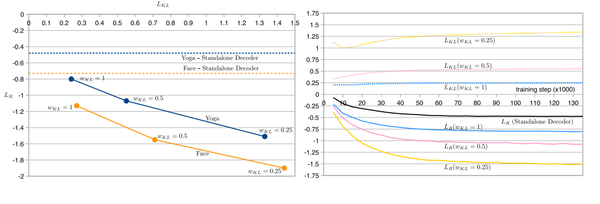
When [math]\displaystyle{ w_{KL} = 0 }[/math], the model becomes a standalone unconditional generator. Specially, there will be no [math]\displaystyle{ L_{KL} }[/math] term as we only optimize for [math]\displaystyle{ L_{R} }[/math]. By removing the [math]\displaystyle{ L_{KL} }[/math] term the model approaches a pure autoencoder, meaning it sacrifices the ability to enforce a prior over the latent space and gains better reconstruction loss metrics.

While the aforementioned loss function could be used, it was found that annealing the KL term (as shown below) in the loss function produces better results.

[math]\displaystyle{ \eta_{step} = 1 - (1 - \eta_{min})R^{step} }[/math] [math]\displaystyle{ Loss_{train} = L_R + w_{KL} \eta_{step} max(L_{KL}, KL_{min}) }[/math]

As shown in Figure 4, the [math]\displaystyle{ L_{R} }[/math] metric for the standalone decoder model is actually an upper bound for different models using a latent vector. The reason is the unconditional model does not access to the entire sketch it needs to generate.

Figure 4. Tradeoff between [math]\displaystyle{ L_{R} }[/math] and [math]\displaystyle{ L_{KL} }[/math], for two models trained on single class datasets (left). Validation Loss Graph for models trained on the Yoga dataset using various [math]\displaystyle{ w_{KL} }[/math]. (right)

Experiments

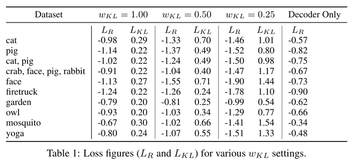
The authors experiment with the sketch-rnn model using different settings and recorded both losses. They used a Long Short-Term Memory(LSTM) model as an encoder and a HyperLSTM as a decoder. HyperLSTM is a type of RNN cell that excels at sequence generation tasks. The ability for HyperLSTM to spontaneously augment its own weights enables it to adapt to many different regimes in a large diverse dataset. They also conduct multi-class datasets. The result is as follows.

We could see the trade-off between [math]\displaystyle{ L_R }[/math] and [math]\displaystyle{ L_{KL} }[/math] in this table clearly. Furthermore, [math]\displaystyle{ L_R }[/math] decreases as [math]\displaystyle{ w_{KL} }[/math] is halfed.

Conditional Reconstruction

The authors assess the reconstructed sketch with a given sketch with different [math]\displaystyle{ \tau }[/math] values. We could see that with high [math]\displaystyle{ \tau }[/math] value on the right, the reconstructed sketches are more random.

They also experiment on inputting a sketch from a different class. The output will still keep some features from the class that the model is trained on.

Latent Space Interpolation

The authors visualize the reconstruction sketches while interpolating between latent vectors using different [math]\displaystyle{ w_{KL} }[/math] values. With high [math]\displaystyle{ w_{KL} }[/math] values, the generated images are more coherently interpolated.

Sketch Drawing Analogies

Since the latent vector [math]\displaystyle{ z }[/math] encode conceptual features of a sketch, those features can also be used to augment other sketches that do not have these features. This is possible when models are trained with low [math]\displaystyle{ L_{KL} }[/math] values. The authors are able to perform vector arithmetic on latent vectors from different sketches and explore how the model generates sketches base on these latent spaces.

Predicting Different Endings of Incomplete Sketches

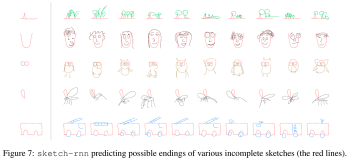
This model is able to predict an incomplete sketch by encoding the sketch into hidden state [math]\displaystyle{ h }[/math] using the decoder and then using [math]\displaystyle{ h }[/math] as an initial hidden state to generate the remaining sketch. The authors train on individual classes by using decoder-only models and set τ = 0.8 to complete samples. Figure 7 shows the results.

Limitations

Although sketch-rnn can model a large variety of sketch drawings, there are several limitations in the current approach.

Applications and Future Work

The authors believe this model can assist artists by suggesting how to finish a sketch, helping them to find interesting intersections between different drawings or objects, or generating a lot of similar but different designs. In the simplest use, pattern designers can apply sketch-rnn to generate a large number of similar, but unique designs for textile or wallpaper prints. The creative designers can also come up with abstract designs which enables them to resonate more with their target audience

This model may also find its place on teaching students how to draw. Even with the simple sketches in QuickDraw, the authors of this work have become much more proficient at drawing animals, insects, and various sea creatures after conducting these experiments. When the model is trained with a high [math]\displaystyle{ w_{KL} }[/math] and sampled with a low [math]\displaystyle{ \tau }[/math], it may help to turn a poor sketch into a more aesthetical one. Latent vector augmentation could also help to create a better drawing by inputting user-rating data during training processes.

The authors conclude by providing the following future directions to this work:

1. Investigate using user-rating data to augmenting the latent vector in the direction that maximizes the aesthetics of the drawing.
2. Look into combining variations of sequence-generation models with unsupervised, cross-domain pixel image generation models.

It's exciting that they manage to combine this model with other unsupervised, cross-domain pixel image generation models to create photorealistic images from sketches.

The authors have also mentioned the opposite direction of converting a photograph of an object into an unrealistic, but similar looking sketch of the object composed of a minimal number of lines to be a more interesting problem.

Moreover, it would be interesting to see how varying loss will be represented as a drawing. Some exotic form of loss function may change the way that the network behaves, which can lead to various applications.

Conclusion

The paper presents a methodology to model sketch drawings using recurrent neural networks. The sketch-rnn model that can encode and decode sketches, generate and complete unfinished sketches is introduced in this paper. In addition, Authors demonstrated how to both interpolate between latent spaces from a different class, and use it to augment sketches or generate similar looking sketches. Furthermore, the importance of enforcing a prior distribution on latent vector while interpolating coherent sketch generations is shown. Finally, a large sketch drawings dataset for future research work is created.

Critique

This paper presents both a novel large dataset of sketches and a new RNN architecture to generate new sketches. It is very exciting to read but there are stil some aspect to improve.

• The performance of the decoder model can hardly be evaluated. The authors present the performance of the decoder by showing the generated sketches, it is clear and straightforward, however, not very efficient. It would be great if the authors could present a way, or a metric to evaluate how well the sketches are generated rather than printing them out and evaluate with human judgment. The authors didn't present an evaluation of the algorithms either. They provided [math]\displaystyle{ L_R }[/math] and [math]\displaystyle{ L_{KL} }[/math] for reference, however, a lower loss doesn't represent a better performance. Training loss alone likely does not capture the quality of a sketch.

• Algorithm lacks comparison to the prior state of the art on standard metrics, which made the novelty unclear. Using strokes as inputs is a novel and innovative move, however, the paper does not provide a baseline or any comparison with other methods or algorithms. Some other researches were mentioned in the paper, using similar and smaller datasets. It would be great if the authors could use some basic or existing methods a baseline and compare with the new algorithm.

• Besides the comparison with other algorithms, it would also be great if the authors could remove or replace some component of the algorithm in the model to show if one part is necessary, or what made them decide to include a specific component in the algorithm.

• The authors proposed a few future applications for the model, however, the current output seems somehow not very close to their descriptions. But I do believe that this is a very good beginning, with the release of the sketch dataset, it must attract more scholars to research and improve with it!

References

1. Jimmy L. Ba, Jamie R. Kiros, and Geoffrey E. Hinton. Layer normalization. NIPS, 2016.
2. Christopher M. Bishop. Mixture density networks. Technical Report, 1994. URL http://publications.aston.ac.uk/373/.
3. Samuel R. Bowman, Luke Vilnis, Oriol Vinyals, Andrew M. Dai, Rafal Józefowicz, and Samy Bengio. Generating Sentences from a Continuous Space. CoRR, abs/1511.06349, 2015. URL http://arxiv.org/abs/1511.06349.
4. H. Dong, P. Neekhara, C. Wu, and Y. Guo. Unsupervised Image-to-Image Translation with Generative Adversarial Networks. ArXiv e-prints, January 2017.
5. David H. Douglas and Thomas K. Peucker. Algorithms for the reduction of the number of points required to represent a digitized line or its caricature. Cartographica: The International Journal for Geographic Information and Geovisualization, 10(2):112–122, October 1973. doi: 10.3138/fm57-6770-u75u-7727. URL http://dx.doi.org/10.3138/fm57-6770-u75u-7727.
6. Mathias Eitz, James Hays, and Marc Alexa. How Do Humans Sketch Objects? ACM Trans. Graph.(Proc. SIGGRAPH), 31(4):44:1–44:10, 2012.
7. I. Goodfellow. NIPS 2016 Tutorial: Generative Adversarial Networks. ArXiv e-prints, December 2016.
8. Alex Graves. Generating sequences with recurrent neural networks. arXiv:1308.0850, 2013.
9. David Ha. Recurrent Net Dreams Up Fake Chinese Characters in Vector Format with TensorFlow, 2015.
10. David Ha, Andrew M. Dai, and Quoc V. Le. HyperNetworks. In ICLR, 2017.
11. Sepp Hochreiter and Juergen Schmidhuber. Long short-term memory. Neural Computation, 1997.
12. P. Isola, J.-Y. Zhu, T. Zhou, and A. A. Efros. Image-to-Image Translation with Conditional Adversarial Networks. ArXiv e-prints, November 2016.
13. Jonas Jongejan, Henry Rowley, Takashi Kawashima, Jongmin Kim, and Nick Fox-Gieg. The Quick, Draw! - A.I. Experiment. https://quickdraw.withgoogle.com/, 2016. URL https: //quickdraw.withgoogle.com/.
14. C. Kaae Sønderby, T. Raiko, L. Maaløe, S. Kaae Sønderby, and O. Winther. Ladder Variational Autoencoders. ArXiv e-prints, February 2016.
15. T. Kim, M. Cha, H. Kim, J. Lee, and J. Kim. Learning to Discover cross-domain Relations with Generative Adversarial Networks. ArXiv e-prints, March 2017.
16. D. P Kingma and M. Welling. Auto-Encoding Variational Bayes. ArXiv e-prints, December 2013.
17. Diederik Kingma and Jimmy Ba. Adam: A method for stochastic optimization. In ICLR, 2015.
18. Diederik P. Kingma, Tim Salimans, and Max Welling. Improving variational inference with inverse autoregressive flow. CoRR, abs/1606.04934, 2016. URL http://arxiv.org/abs/1606.04934.
19. Brenden M. Lake, Ruslan Salakhutdinov, and Joshua B. Tenenbaum. Human level concept learning through probabilistic program induction. Science, 350(6266):1332–1338, December 2015. ISSN 1095-9203. doi: 10.1126/science.aab3050. URL http://dx.doi.org/10.1126/science.aab3050.
20. Yong Jae Lee, C. Lawrence Zitnick, and Michael F. Cohen. Shadowdraw: Real-time user guidance for freehand drawing. In ACM SIGGRAPH 2011 Papers, SIGGRAPH ’11, pp. 27:1–27:10, New York, NY, USA, 2011. ACM. ISBN 978-1-4503-0943-1. doi: 10.1145/1964921.1964922. URL http://doi.acm.org/10.1145/1964921.1964922.
21. M.-Y. Liu, T. Breuel, and J. Kautz. Unsupervised Image-to-Image Translation Networks. ArXiv e-prints, March 2017.
22. S. Reed, A. van den Oord, N. Kalchbrenner, S. Gómez Colmenarejo, Z. Wang, D. Belov, and N. de Freitas. Parallel Multiscale Autoregressive Density Estimation. ArXiv e-prints, March 2017.
23. Patsorn Sangkloy, Nathan Burnell, Cusuh Ham, and James Hays. The Sketchy Database: Learning to Retrieve Badly Drawn Bunnies. ACM Trans. Graph., 35(4):119:1–119:12, July 2016. ISSN 0730-0301. doi: 10.1145/2897824.2925954. URL http://doi.acm.org/10.1145/2897824.2925954.
24. Mike Schuster, Kuldip K. Paliwal, and A. General. Bidirectional recurrent neural networks. IEEE Transactions on Signal Processing, 1997.
25. Saul Simhon and Gregory Dudek. Sketch interpretation and refinement using statistical models. In Proceedings of the Fifteenth Eurographics Conference on Rendering Techniques, EGSR’04, pp. 23–32, Aire-la-Ville, Switzerland, Switzerland, 2004. Eurographics Association. ISBN 3-905673-12-6. doi: 10.2312/EGWR/EGSR04/023-032. URL http://dx.doi.org/10.2312/EGWR/EGSR04/023-032.
26. Patrick Tresset and Frederic Fol Leymarie. Portrait drawing by paul the robot. Comput. Graph.,37(5):348–363, August 2013. ISSN 0097-8493. doi: 10.1016/j.cag.2013.01.012. URL http://dx.doi.org/10.1016/j.cag.2013.01.012.
27. T. White. Sampling Generative Networks. ArXiv e-prints, September 2016.
28. Ning Xie, Hirotaka Hachiya, and Masashi Sugiyama. Artist agent: A reinforcement learning approach to automatic stroke generation in oriental ink painting. In ICML. icml.cc / Omnipress, 2012. URL http://dblp.uni-trier.de/db/conf/icml/icml2012.html#XieHS12.
29. Xu-Yao Zhang, Fei Yin, Yan-Ming Zhang, Cheng-Lin Liu, and Yoshua Bengio. Drawing and Recognizing Chinese Characters with Recurrent Neural Network. CoRR, abs/1606.06539, 2016. URL http://arxiv.org/abs/1606.06539.