stat841

Course Note for Sept.30th (Classfication_by Liang Jiaxi)

1. Review of LLE

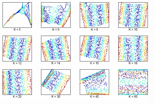
The size of neighborhood chosen in LLE influences the effect of LLE. The picture above shows the effect of neighborhood size to LLE of the two dimensional S-manifold in the top panels. We can lower dimension from D=3 to d=2 by choosing K nearest neighbors. Apparently, when K is too small or too large, the LLE fails to find out the two main degree of freedom.

2. Classification
A 'classification rule' [math]\displaystyle{ \,h }[/math] is a function between two discrete random variables [math]\displaystyle{ \,X }[/math] and [math]\displaystyle{ \,Y }[/math]. Given n pairs of data [math]\displaystyle{ \,(X_{1},Y_{1}), (X_{2},Y_{2}), \dots , (X_{n},Y_{n}) }[/math], where [math]\displaystyle{ \,X_{i}= \{ X_{i1}, X_{i2}, \dots , X_{id} \} \in \mathcal{X} \subset \Re^{d} }[/math]
is a d-dimensional vector and [math]\displaystyle{ \,Y_{i} }[/math] takes values in a finite set [math]\displaystyle{ \, \mathcal{Y} }[/math]. Set up a function [math]\displaystyle{ \,h }[/math] that [math]\displaystyle{ \,h: \mathcal{X} \mapsto \mathcal{Y} }[/math]. Thus, given a new vector [math]\displaystyle{ \,X }[/math], we can give a prediction of corresponding [math]\displaystyle{ \,Y }[/math] by the classification rule [math]\displaystyle{ \,h }[/math] that [math]\displaystyle{ \,\overline{Y}=h(X) }[/math]

Example Suppose we wish to classify fruit into apples and oranges by considering certain features of the fruit. Let [math]\displaystyle{ \mathcal{X}_{i} }[/math]= (colour, diameter, weight) for fruit i and [math]\displaystyle{ \mathcal{Y} }[/math]={apple, orange}. The goal is to find a classification rule such that when a new fruit [math]\displaystyle{ \mathcal{X} }[/math] is presented, it can be classified as either an apple or an orange.

3. Error data
Definition:
'True error rate' of a classifier(h) is defined as the probability that [math]\displaystyle{ \overline{Y} }[/math] predicted from [math]\displaystyle{ \,X }[/math] by classifier [math]\displaystyle{ \,h }[/math] does not actually equal to [math]\displaystyle{ \,Y }[/math], namely, [math]\displaystyle{ \, L(h)=P(h(X) \neq Y) }[/math].
'Empirical error rate(training error rate)' of a classifier(h) is defined as the frequency that [math]\displaystyle{ \overline{Y} }[/math] predicted from [math]\displaystyle{ \,X }[/math] by [math]\displaystyle{ \,h }[/math] does not equal [math]\displaystyle{ \,Y }[/math] in n predictions. The mathematical expression is as below:
[math]\displaystyle{ \, L_{h}= \frac{1}{n} \sum_{i=1}^{n} I(h(X_{i}) \neq Y_{i}) }[/math], where [math]\displaystyle{ \,I }[/math] is an indicator that [math]\displaystyle{ \, I= \left\{\begin{matrix} 1 & h(X_i) \neq Y_i \\ 0 & h(X_i)=Y_i \end{matrix}\right. }[/math].

4. Bayes Classifier
Consider the special case that [math]\displaystyle{ \,Y }[/math] has only two possible values, that is, [math]\displaystyle{ \, \mathcal{Y}=\{0, 1\} }[/math]. Consider the probability that [math]\displaystyle{ \,r(X)=P\{Y=1|X=x\} }[/math]. Given [math]\displaystyle{ \,x }[/math], if [math]\displaystyle{ \,P(Y=1|X=x)\gt P(Y=0|X=x) }[/math], then [math]\displaystyle{ \,Y }[/math] is more likely to be 1 when [math]\displaystyle{ \,X=x }[/math]. But since [math]\displaystyle{ \, 0, 1 \in \mathcal{Y} }[/math] is labels, it is meaningless to measure the conditional prabobility of [math]\displaystyle{ \,Y }[/math]. Thus, by Bayes formula, we have
[math]\displaystyle{ \,r(X)=P(Y=1|X=x)=\frac{P(X=x|Y=1)P(Y=1)}{P(X=x)}=\frac{P(X=x|Y=1)P(Y=1)}{P(X=x|Y=1)P(Y=1)+P(X=x|Y=0)P(Y=0)} }[/math]

Definition:
The Bayes classification rule [math]\displaystyle{ \,h }[/math] is:
[math]\displaystyle{ \, h(X)= \left\{\begin{matrix} 1 & r(x)\gt \frac{1}{2} \\ 0 & otherwise \end{matrix}\right. }[/math]

The set [math]\displaystyle{ \,D(h)=\{x: P(Y=1|X=x)=P(Y=0|X=x)\} }[/math] is called the decision boundary

'Important Theorem': The Bayes rule is optimal in true error rate, that is for any other classification rule [math]\displaystyle{ \, \overline{h} }[/math], we have [math]\displaystyle{ \,L(\overline{h}) \le L(h) }[/math].

Notice: Although the Bayes rule is optimal, we still need other methods, and the reason for the fact is that in the Bayes equation discussed before, it is generally impossible for us to know the [math]\displaystyle{ \,P(Y=1) }[/math], and [math]\displaystyle{ \,P(X=x|Y=1) }[/math] and ultimately calculate the value of [math]\displaystyle{ \,r(X) }[/math], which makes Bayes rule inconvenient in practice.