Gradient Episodic Memory for Continual Learning
Presented by
- Yu Xuan Lee
- Tsen Yee Heng
Background and Introduction
Supervised learning consist of a training set [math]\displaystyle{ D_{tx}=(x_i,y_i)^n_{i=1} }[/math], where [math]\displaystyle{ x_i \in \mathcal{X} }[/math] and [math]\displaystyle{ y_i \in \mathcal{Y} }[/math]. Empirical Risk Minimization (ERM) is one of the common supervised learning method used to minimize a loss function by having multiple passes over the training set.
- [math]\displaystyle{ \frac{1}{|D_{tr}|}\textstyle \sum_{(x_i,y_i) \in D_{tr}} \ell (f(x_i),y_i) }[/math]
where [math]\displaystyle{ \ell :\mathcal {Y} \times \mathcal {Y} \to [0, \infty) }[/math]
Different to machine learning, datas are being observed sequentially, occurred recurrently, and stored limitedly for learning humans. Thus, the iid assumption is not applicable to ERM. One of the characteristics of ERM is "catastrophic forgetting", which is the problem of recalling past knowledge upon acquiring new ones. To overcome this problem, Gradient Episodic Memory (GEM) is introduced to alleviates forgetting on previous acquired knowledge, while solving new problems more efficiently.
Framework for Continual Learning
The feature vector [math]\displaystyle{ x_i \in \mathcal{X}_t }[/math], task descriptor [math]\displaystyle{ t_i \in \mathcal{T} }[/math], and target vector [math]\displaystyle{ y_i \in \mathcal{Y}_t }[/math] are the three main components of a continuum of data. Note that the continuum is locally iid where for every [math]\displaystyle{ (x_i, t_i, y_i) }[/math]
- [math]\displaystyle{ (x_i,y_i) \overset{iid}{\sim} P_{t_i}(X,Y) }[/math]
The main mathematical purpose of continual learning is to obtain [math]\displaystyle{ f: \mathcal{X} \times \mathcal{Y} }[/math] where a target vector [math]\displaystyle{ y }[/math] must be inquired using a test pair [math]\displaystyle{ (x,t) }[/math].
Task Descriptor
Task descriptors are structured objects, describing how to solve each [math]\displaystyle{ i }[/math]-th task. They are integers [math]\displaystyle{ t_i=i \in \mathbb{Z} }[/math] which occurs in a collection where [math]\displaystyle{ t_1,...,t_n \in \mathcal{T} }[/math]. Most importantly, they could distinguish every same input [math]\displaystyle{ x_i }[/math] that have different target. To conclude, task descriptors plays the part of carrying crucial information of the example and distinguishing different learning environment for similar examples.
Training Protocol
The target setting for continual learning are as follow:
- Large task quantity
- Small quantity of training examples for each task
- Examples for each tasks being observed only once
- Outcome of transfer and forgetting being concluded
To perform this, each example were only given once to the learner in one at a time in sequence. In this case, learner gets information in [math]\displaystyle{ (x_i,t_i,y_i) }[/math] form with no duplication.
Evaluation Metrics
The capability of transferring knowledge across tasks are very important in addition to results across each tasks. First of all, transferring knowledge are categorized as follow:
- Backward transfer (BWT) This is the difference of judgement towards previously encountered task [math]\displaystyle{ k }[/math] after learning new task [math]\displaystyle{ t }[/math], noted as [math]\displaystyle{ k \prec t }[/math]. Within backward transfer, there are two categories, positive backward transfer and negative backward transfer. Positive backward transfer shows a better judgement towards previously encountered task [math]\displaystyle{ k }[/math] after learning new task [math]\displaystyle{ t }[/math]. Contrarily, negative backward transfer shows the opposite. Also, do note that catastrophic forgetting happens due to extensive negative backward transfer.
- Forward transfer (FWT) Opposite to BWT, FWT shows judgement towards new task [math]\displaystyle{ t }[/math] after learning task [math]\displaystyle{ k }[/math], noted as [math]\displaystyle{ k \succ t }[/math]. Positive forward transfer is one way of forward transfer.
Given a test set of [math]\displaystyle{ T }[/math], we would learn task [math]\displaystyle{ t_i }[/math] and observe its performance towards all [math]\displaystyle{ T }[/math] tasks. A matrix [math]\displaystyle{ R_{i,j} }[/math] as test classification accuracy of the model on task [math]\displaystyle{ t_j }[/math] after observing the last sample from task [math]\displaystyle{ t_j }[/math] is constructed, where [math]\displaystyle{ R \in \mathbb{R} ^{T \times T} }[/math]. Note that [math]\displaystyle{ \bar b\ }[/math] is the vector of test accuracies for each task at random initialization. The function for Average Accuracy (ACC), Backward Transfer (BWT) and Forward Transfer (FWT) are shown below:
- [math]\displaystyle{ ACC = \frac{1}{T} \sum_{i=1}^T R_{T,i} }[/math]
- [math]\displaystyle{ BWT = \frac{1}{T-1} \sum_{i=1}^{T-1} R_{T,i} - R_{i,i} }[/math]
- [math]\displaystyle{ FWT = \frac{1}{T-1} \sum_{i=2}^{T} R_{i-1,i- \bar b\ _i} }[/math]
Note that if ACC happens to be similar for both models, model with higher BWT and FWT values are more desired.
Gradient Episodic Memory (GEM)
Episodic memory [math]\displaystyle{ M_t }[/math] is very important in GEM, it contains information on examples on task [math]\displaystyle{ t }[/math] and it is indicated from the integer task descriptors. So practically, we would minimize catastrophic forgetting by using the episodic memory efficiently. Note that learner is assumed to have limited memory locations [math]\displaystyle{ M }[/math]. Hence, the amount located for each task is calculated as [math]\displaystyle{ m=\frac{M}{T} }[/math] which results to more memory for the final [math]\displaystyle{ m }[/math] examples for each tasks. To calculate the loss of memories from the [math]\displaystyle{ k }[/math]-th task, assuming predictors [math]\displaystyle{ f_ \theta }[/math] parameterized by [math]\displaystyle{ \theta \in \mathbb{R} ^p }[/math], we have the following equation:
- [math]\displaystyle{ \ell (f_\theta, \mathcal{M}_k)=\frac{1}{|\mathcal{M}_k|} \sum_{(x_i,k,y_i) \in \mathcal{M}_k} \ell(f_ \theta (x_i,k),y_i) }[/math]
The above equation will be treated as inequality constraint and a decrease in the equation would be in favour instead of increase. So we would use [math]\displaystyle{ (x,t,y) }[/math] to minimize the following equation:
- [math]\displaystyle{ mimimize_\theta \space \space \ell(f_\theta(x,t),y) }[/math]
- [math]\displaystyle{ subject\space to \space \space \ell (f_\theta,\mathcal{M}_k) \le \ell(f_\theta^{t-1},\mathcal{M}_k) \space\space for \space all \space k\lt t }[/math]
where [math]\displaystyle{ f_\theta^{t-1} }[/math] is the predictor state at the end of learning of task [math]\displaystyle{ t-1 }[/math].
To efficiently solve the above equation, three ideas are proposed:
- Delete old predictors [math]\displaystyle{ f_\theta^{t-1} }[/math]. This is because the old predictors remain unchanged for each update of g.
- Functions are locally linear.
- Loss of previous tasks could be calculated using the angle between loss gradient vector and proposed update.
With the above ideas, the loss function is further improved as follow:
- [math]\displaystyle{ \langle g,g_k \rangle := \langle \frac{\partial \ell(f_\theta(x,t),y)}{\partial \theta}, \frac{\partial \ell(f_\theta,\mathcal{M}_k)}{\partial \theta} \rangle \ge 0, \space for \space all \space k\lt t. }[/math]
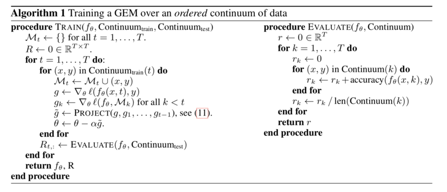
However, if there is at least one violation in the equality constraint, we would overcome this by projecting the gradient [math]\displaystyle{ g }[/math] to the closest gradient [math]\displaystyle{ \tilde{g} }[/math] satisfying all the constraints. The optimization problem becomes
- [math]\displaystyle{ minimize_{ \tilde{g} } \space \space \frac{1}{2}\parallel g - \tilde{g} \parallel _2^2 }[/math]
- [math]\displaystyle{ subject \space to \space \space \langle \tilde{g},g_k \rangle \ge 0 \space \space for \space all \space k\lt t }[/math]
Therefore, the primal GEM Quadratic Program (QP) is
- [math]\displaystyle{ minimize_z \space \space \frac{1}{2}z^Tz - g^Tz+\frac{1}{2}g^Tg }[/math]
- [math]\displaystyle{ subject \space to \space \space Gz \ge 0, }[/math]
Dual of the GEM QP is
- [math]\displaystyle{ minimize_v \space \space \frac{1}{2}v^TGG^Tv + g^TG^Tv }[/math]
- [math]\displaystyle{ subject \space to \space \space v\ge 0 }[/math]
By solving [math]\displaystyle{ v^* }[/math], we could obtain the projected gradient update [math]\displaystyle{ \tilde{g}=G^Tv^* + g }[/math]. The algorithm is as follow:
Experiment
We perform a variety of experiments to assess the performance of GEM in continual learning.
Dataset
We consider the following dataset:
- MNIST Permutations It is a variant of MNIST dataset of handwritten digits, where each task is transformed by a fixed permutation of pixels.
In this dataset, the input distribution for each task is unrelated.
- MNIST Rotation It is a variant of MNIST where each task contain digits rotated by a fixed angle between 0 and 180 degree.
- CIFAR100 It is a variant of CIFAR dataset with 100 classes, which each task introduces a new set of classes. For a total of T tasks, each new task concerns examples from a disjoint subset of 100/T classes. Here, the input distribution is similar for all task, but different task required different output distribution.
For all the datasets, we consider T = 20 tasks. On the MNIST dataset, each task has 1000 samples from 10 different classes and for the CIFAR datasets, each task has 2500 examples from 5 different classes. The model observe the task in sequence, and each example once.
Architectures
On the MNIST tasks, we use fully-connected neural network with two hidden layers of 100 ReLU units. On the CIFAR tasks, we use a smaller version of ResNet18, with three times less feature maps across all layers. Also on CIFAR, the network has a final linear classifier per task. This is one simple way to leverage the task descriptor, in order to adapt the output distribution to the subset of classes for each task. we train all the networks and baselines using plain SGD on mini batches of 10 samples. All hyper-parameter are optimized using grid-search, and the best result for each model are reported.
Methods
We compare GEM to 5 alternatives:
- 1. a single predictor trained across all tasks.
- 2. one independent predictor for each task. Each of them has the same architecture as "single" but with T times less hidden units than "single". Each of them are initialized at random , or be a clone of the last trained predictor(decided by grid-search).
- 3. a multimodal predictor, which has the same architecture as "single", but with a dedicated input layer per task (only for MNIST).
- 4. EWC, where the loss is regularized to avoid catastrophic forgetting.
- 5. iCARL, a class-incremented learner that classifies using a nearest exemplar algorithm, and using an episodic memory to prevent catastrophic forgetting. iCARL required the same input representation across tasks, so this method only applied to our experement on CIFAR100.
Notes : GEM, EWC, iCARL has the same architecture as "single", with episodic memory.
Results
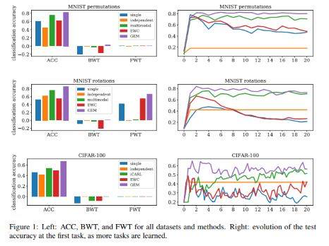
Figure 1 (left) shows the average accuracy, BWT and FWT. Overall, GEM performs similarly or better than multimodal model( well suited to the MNIST tasks). GEM minimized backward transfer , while exhibiting negligible or positive forward transfer.
Figure 1(right) shows the evolution of the test accuracy of the first task throughout the continuum of data. GEM exhibits minimal forgetting, and achieve positive BWT in CIFAR100.
Overall, GEM performs slightly better than other continuing method like EWC, while spending less computational. GEM efficiency comes from optimizing over a number of variables equal to the number of tasks, instead of optimizing over a number of variables equal to the number of parameters.
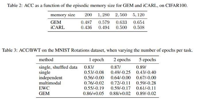
Table 2 shows the final ACC for both GEM and iCARL in the dataset CIFAR100, as a function of their episodic memory size. As we can see from table 2, GEM outperform iCARL for a wide range of memory sizes.
Table 3 shows that the importance of memory as we do more than one pass through the data on the MNIST Rotation experiment. As we can see from table 3, memory based method such as GEM and EWC lead to a higher ACC as in number of passes through the data increases, and memory-less method exhibits higher negative BWT, which has lower accuracy. By comparing the first and last row of table 3, GEM matches the “oracle performance upper-bound” ACC provided by iid learning, and minimizes negative BWT, which has higher ACC.
Related Work
Continual learning is a method which retain knowledge about past tasks and leverage that knowledge to quickly acquire new skills through all the tasks. This learning setting led to implementation and theoretical investigations, although the latter ones have been restricted to linear model. In this work, we use continuing learning to focus more on the realistic setting where examples are only seen once. Thus, we introduced the GEM, which outperforms every model in limiting forgetting.
There are some ways to avoid catastrophic forgetting. The simple one is to freeze the early layer in the neural network and duplicate the later layers on new tasks. However, it is hard to scale up these methods and there are too many modules and tasks. Our approach is to use a single model and modify its learning objective to avoid catastrophic forgetting. There is some method which use synaptic memory, which minimized the important parameters for the previous task. Other method which use episodic memory stored and replayed the examples from previous tasks to prevent forgetting which allow positive backward transfer.
Conclusion
The scenario of continuing learning is being formalized. Firstly, the training and evaluation protocol are being defined to assess the quality of models in term of their accuracy, and the ability to transfer knowledge with BWT and FWT. Secondly, GEM is introduced as a model which leverage the episodic memory to get a positive BWT and avoid forgetting efficiently. We demonstrate the effectiveness of GEM by comparing to other model such as EWC, multimodal, etc.
However, there is some improvement has to be done to GEM. Firstly, GEM might obtain positive FWT because it do not leverage structured task descriptor. Secondly, there are too many complicated structures in advance memory management which we did not investigate. Thirdly, the iteration of GEM increase the computational time.


