neighbourhood Components Analysis

Introduction

Neighbourhood Components Analysis (NCA) is a method for learning a Mahalnobis distance measure for k-nearest neighbours (KNN). In particular, it finds a distance metric that maximises the leave one out (LOO) error on the training set for a stochastic variant of KNN. NCA can also learn a low-dimensional linear embedding of labelled data for data visualisation and for improved KNN classification speed. Unlike other methods, this classification model is non-parametric without any assumption on the shape of the class distributions or the boundaries between them.

k-Nearest Neighbours

k-Nearest neighbors is a simple classification technique that determines a test point's label by looking at the labels of the [math]\displaystyle{ \,k }[/math] training points that are nearest the test point. This is a surprisingly effective method that has a non-linear decision surface that is non-parametric, except for the parameter [math]\displaystyle{ k }[/math].

However, KNN suffers from two problems. First, it can be computationally expensive to classify points as they must be stored and compared over the entire training set. There is also the problem of determining which distance metric is to be used to define "nearest" points.

Stochastic Nearest Neighbours

NCA attacks the above two problems of KNN. It finds a quadratic distance metric that defines which points are nearest. It can restrict this distance metric to be low rank, reducing the dimensionality of the data and thus reducing storage and search times.

Starting with a labeled dataset [math]\displaystyle{ x_1, x_2, ..., x_n \in R^D }[/math] and corresponding class labels [math]\displaystyle{ \,\!c_1, c_2, ..., c_n }[/math], we are looking for a distance metric that maximizes the performance of nearest neighbor classification. As we do not knw the actual future data, optimizing Leave-one-out performance on the training data can be substituted.

NCA finds the matrix [math]\displaystyle{ A }[/math] where [math]\displaystyle{ \,Q = A^{T} A }[/math] and distance between two points is defined as: [math]\displaystyle{ \,d(x,y) = (x - y)^T Q(x - y) = (Ax - Ay)^T (Ax - Ay) }[/math].

The basic idea of NCA is to find the distance metric [math]\displaystyle{ \,A }[/math] that maximizes the KNN classification on test data. As test data is not available during training, the method uses Leave One Out (LOO) performance. However, KNN has a discontinuous error function as points can suddenly jump class as they cross class boundaries. Instead, NCA optimises using stochastic neighbour assignment. Here, a test point is assigned a neighbour (and the neighbour's class) according to probability [math]\displaystyle{ p_{ij} }[/math]. This probability decreases as the distance between points increases: [math]\displaystyle{ p_{ij} = \frac{exp(-\parallel Ax_i - Ax_j \parallel ^2)}{\sum_{k \neq i}exp(-\parallel Ax_i - Ax_k \parallel ^2)} }[/math] , [math]\displaystyle{ \textstyle p_{ii} = 0 }[/math].

Here, for a single point every point in the training set is considered to be it's neighbour but with different probabilities and the probability of that point being the neighbour of itself is considered to be zero. And, in this sense it becomes a leave one out classification.

This stochastic selection rule helps us find the probability [math]\displaystyle{ p_i }[/math] that point [math]\displaystyle{ i }[/math] will be correctly classified:
[math]\displaystyle{ p_i = \sum_{j\in c_i} p_{ij} }[/math] where [math]\displaystyle{ c_i=\{j|c_i=c_j\} }[/math]
NCA maximises the expected number of correctly classified points according to this objective function:

[math]\displaystyle{ f(A) = \sum_i \sum_{j \in C_i} p_{ij} = \sum_i p_i }[/math]

The gradient for which is easily found:

[math]\displaystyle{ \frac{\partial f}{\partial A} = 2A \sum_i \left( p_i \sum_k p_{ik} x_{ik} x_{ik}^T - \sum_{j \in C_i} p_{ij} x_{ij} x_{ij}^T \right) }[/math]

NCA then finds A using a gradient-based optimizer. Note, however, that the cost function is not convex, so the optimization must handle local minima. The authors comment that they never observed any effects of over fitting in this method, and that performance never decreased as the training set size increased.

It is possible to use a cost function based on KL-divergence, and the authors note that performance is very similar to that achieved through the above cost function. The cost function based on KL divergence is:

[math]\displaystyle{ g(A)=\sum_i \log(\sum_{j \in C_i} p_{ij})=\sum_i \log(p_i) }[/math]

with gradient:

[math]\displaystyle{ \frac{\partial g}{\partial A} = 2A \sum_i \left( \sum_k p_{ik} x_{ik} x_{ik}^T - \frac{\sum_{j \in C_i} p_{ij} x_{ij} x_{ij}^T}{\sum_{j \in C_i} p_{ij} } \right) }[/math]

The scale of [math]\displaystyle{ A }[/math] found by NCA, and relative row directions can provide an estimate to the optimal number of neighbours to use for KNN. In Stochastic NN, a larger scale A tends to consult average over fewer neighbours, and vice versa.

A short note on Kullback-Leibler divergence

In the paper, the objective function [math]\displaystyle{ g(A) = \sum_i log(p_i) \, }[/math] is derived by taking the Kullback-Leibler divergence(KL divergence) between the true class distribution and the stochastic class distribution induced by [math]\displaystyle{ p_{ij} \, }[/math] via [math]\displaystyle{ A \, }[/math]. In this short subsection, we explain the notion of KL divergence, some of its properties and show how the objective function [math]\displaystyle{ g(A) = \sum_i log(p_i) \, }[/math] results from taking KL divergence between the true class distribution and the stochastic class distribution induced by [math]\displaystyle{ p_{ij} \, }[/math].

In essence, KL divergence is a non-symmetric measure of the difference between two probability distributions [math]\displaystyle{ P \, }[/math] and [math]\displaystyle{ Q \, }[/math]. Non-symmetric here means that the KL divergence of [math]\displaystyle{ Q\, }[/math] from [math]\displaystyle{ P\, }[/math], denoted by [math]\displaystyle{ D_{\mathrm{KL}}(P\|Q) \, }[/math] is in general different from the KL divergence of [math]\displaystyle{ P\, }[/math] from [math]\displaystyle{ Q\, }[/math], denoted by [math]\displaystyle{ D_{\mathrm{KL}}(Q\|P) \, }[/math]. Because of this asymmetry, KL divergence is not a true metric.

The notion of KL divergence comes from information theory and has a very intuitive interpretation under the context of coding theory. An important theorem in coding theory shows that the KL divergence of [math]\displaystyle{ P\, }[/math] from [math]\displaystyle{ Q\, }[/math] is the expected number of extra bits required to code samples from [math]\displaystyle{ Q\, }[/math] when using a code based on [math]\displaystyle{ P\, }[/math], rather than using a code based on [math]\displaystyle{ Q\, }[/math].

For discrete random variables [math]\displaystyle{ P\, }[/math] and [math]\displaystyle{ Q\, }[/math], the KL divergence of [math]\displaystyle{ P\, }[/math] from [math]\displaystyle{ Q\, }[/math] is defined to be

[math]\displaystyle{ D_{\mathrm{KL}}(Q\|P) = \sum_i Q(i) \log \frac{Q(i)}{P(i)} }[/math]

It can be shown that KL divergence is non-negative (Gibb's inequality), with KL divergence equals zero if and only if [math]\displaystyle{ P=Q \, }[/math].

Now we can illustrate how the objective function [math]\displaystyle{ g(A) = \sum_i log(p_i) \, }[/math] arises.

First, we'll show that the KL-divergence for the point [math]\displaystyle{ i\, }[/math] is [math]\displaystyle{ - \log(p_i) \, }[/math].

To see this, let [math]\displaystyle{ Q \, }[/math] be the true class distribution for the point [math]\displaystyle{ i \, }[/math] and let [math]\displaystyle{ P \, }[/math] be the stochastic class distribution for the point [math]\displaystyle{ i \, }[/math] induced by [math]\displaystyle{ p_{ij} \, }[/math]. By a class distribution, we mean that the random variables take discrete values like "in Class 1" or "in Class 14".

Because the true class distribution [math]\displaystyle{ Q \, }[/math] is one at the true class label and zero elsewhere, we see from the definition of [math]\displaystyle{ D_{\mathrm{KL}}(Q\|P) \, }[/math] that there is only one term in the summation, which is [math]\displaystyle{ \log(\frac{1}{P(true class)}) \, }[/math], which is equal to [math]\displaystyle{ - \log(p_i) \, }[/math] because [math]\displaystyle{ p_i \, }[/math] is defined to be the probability that point [math]\displaystyle{ i \, }[/math] will be correctly classified by [math]\displaystyle{ P\, }[/math].

By summing over all points [math]\displaystyle{ i \, }[/math], we get [math]\displaystyle{ - \sum_i log(p_i) \, }[/math]. Now we see that [math]\displaystyle{ g(A)\, }[/math] is just the negative of this.

Low Rank Distance Metrics and Nonsquare Projection

NCA allows for linear dimensionality reduction of the input data. This provides computational advantages and is relatively immune to over fitting.

During the optimization procedure in NCA, the matrix [math]\displaystyle{ \,A }[/math] can be restricted to size [math]\displaystyle{ \,d \times D }[/math], where [math]\displaystyle{ \,d \lt D }[/math]. This forces the learned metric to be low rank, and maps all inputs to [math]\displaystyle{ \,\mathbb{R}^d }[/math].

If [math]\displaystyle{ \,d \ll D }[/math], the storage and search times for KNN will be much lower. Storage can be reduced from [math]\displaystyle{ \,O(DN) }[/math] to [math]\displaystyle{ \,O(dN) + dD }[/math] by storing the training set in the lower-dimensional projection. If [math]\displaystyle{ \,d }[/math] is 2 or 3, then projected points can be easily plotted for data visualization.

The NCA method remains the same as before, optimize the above cost function with respect to [math]\displaystyle{ \,A }[/math], however now [math]\displaystyle{ \,A }[/math] is non-square. Note that NCA itself does not provide suggestions on the optimal size of [math]\displaystyle{ \,d }[/math].

Experimental Results

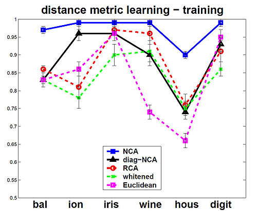
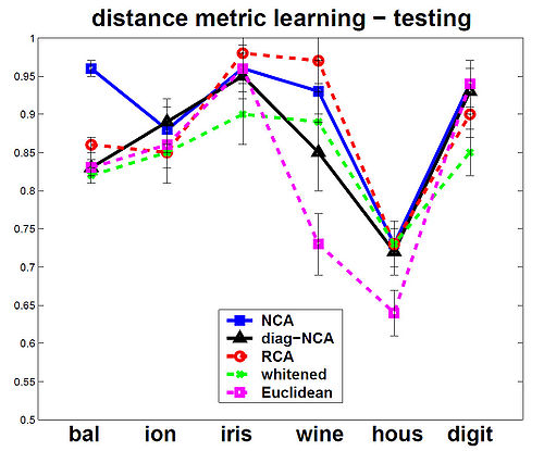
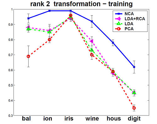
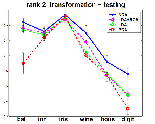
The NCA method was evaluated against the other Mahalanobis measures for KNN distance metrics. Among the six data sets that were used, 5 were from the UCI repository one was a generated data set. In the test, NCA method consistently performed better on training data, and test data performance was always at or near the top as shown in the figures below. The figures below show that the training(on left) and testing performance of NCA (on right) is consistently the same as or better than that of other Mahalanobis distance measures for KNN, despite the relative simplicity of the NCA objective function and the fact that the distance metric being learned is nothing more than a positive definite matrix [math]\displaystyle{ \,A^T A }[/math].The data sets used from UCI repository included balance, ionosphere, iris, wine and housing and on the USPS handwritten digits. Results are the averages over 40 realizations of splitting each dataset into training (70%) and testing (30%) subsets (for USPS 200 images for each of the 10 digit classes were used for training and 500 for testing). Top panels show distance metric learning (square A) and the bottom panels show linear dimensionality reduction down to d = 2.

• 

  distance metric learning - training

• 

  distance metric learning - testing

• 

  rank 2 transformation - training

• 

  rank 2 transformation - testing

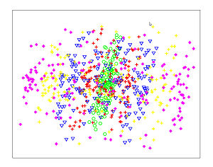
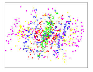
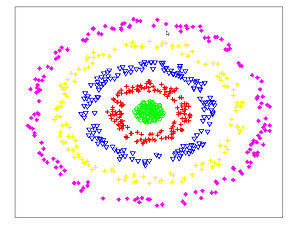
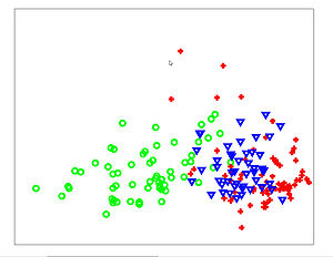
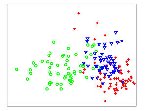
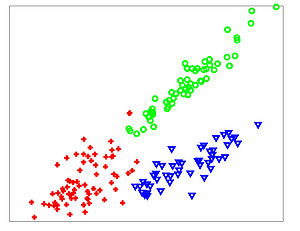
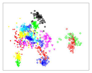
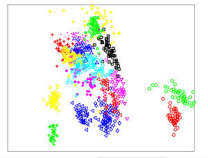
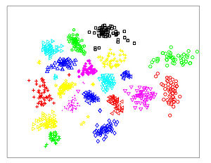
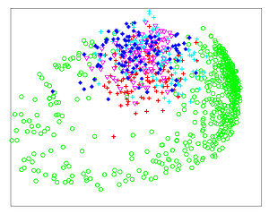
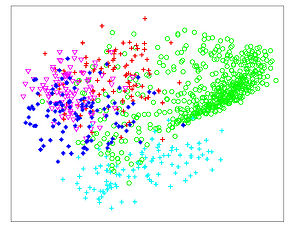
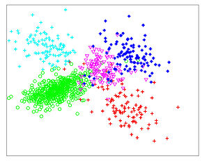
The Figures below show comparison of PCA, LDA, and NCA applied to "concentric ring", "wine", "faces", and "digits" data sets from UCI repository. The output show the reduced dimensionality of d= 2 3 from their original dimensionality which was D = 3 for concentric rings, D = 13 for wine, D = 560 for faces, and D = 256 for digits. Note that NCA produced better 2D projections of the data. Using these 2D projections for classification, NCA performed better consistently for both training and test data. When a two-dimensional projection is used, the classes are consistently much better separated by the NCA transformation than by either PCA, or LDA.

• 

  PCA - Concentric Rings

• 

  LDA - Concentric Rings

• 

  NCA - Concentric Rings

• 

  PCA - Wine

• 

  LDA - Wine

• 

  NCA - Wine

• 

  PCA - Faces

• 

  LDA - Faces

• 

  NCA - Faces

• 

  PCA - Digits

• 

  LDA - Digits

• 

  NCA - Digits

No timing data was provided by the authors.

More Figures are available in the original paper.

Extensions to Continuous Labels and Semi-Supervised Learning

NCA finds a linear transformation to maximise the classification performance on discrete classes. The method can be extended to find a non-linear transformation function [math]\displaystyle{ A }[/math] using the same gradient-based optimisation technique. However, the transformation function must be trainable by gradient methods, such as multilayer perceptrons.

It is also possible to adapt the method to support real-valued, continuous class labelling/targets. Using the above objective function and gradients, define the set [math]\displaystyle{ C_i }[/math] to be a set of correct matches, that is points with similar class labels to [math]\displaystyle{ i }[/math]. The objective function is a weighted sum of points, based on similarity of classes. This allows semi-supervised learning, as target classes need to be explicitly specified, just similarity.

Relationship to Other Methods

Here are other Mahalanobis distance metric learning methods for labelled data. Relevant component analysis (RCA) finds a distance metric, but assumes the classes have Gaussian distributions whereas NCA makes no assumption about class distribution. Xing et al's method finds a transformation that minimises the pairwise distances between points of the same class. This assumes that all points of the one class form a single, compact and connected set. Lowe's method is very similar to NCA, but further constrains the distance metric to be diagonal.

For low rank, linear transformation of data, LDA will be optimal if the classes are Gaussian with common covariance. This is not going to be true in general. LDA also has difficulties with mathematical instability when the training set is small, but the dimensionality of the training data is high. There are newer variants of LDA that improve this instability, and also improve robustness to outliers.