Annotating Object Instances with a Polygon RNN
Summary of the CVPR '17 best paper
Introduction
If a snapshot of an image is given to a human, how will he/she describe a scene? He/she might identify that there is a car parked near the curb, or that the car is parked right besides a street light. This ability to decompose objects in scenes into separate entities is key to understanding what is around us and it helps reason about the behavior of objects in the scene.
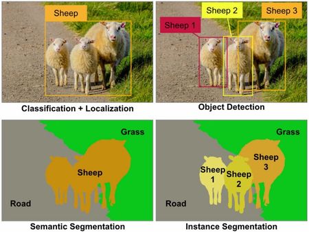
Automating this process is a classic computer vision problem and is often termed "object detection." The term object detection has been used interchangeably, however, there are four distinct levels of detection (refer to Figure 1 for a visual cue):
1. Classification + Localization: This is the most basic method that detects whether an object is either present of absent in the image and then identifies the position of the object within the image in the form of a bounding box overlayed on the image.
2. Object Detection: The classic definition of object detection points to the detection and localization of multiple objects of interest in the image. The output of the detection is still a bounding box overlayed on the image at the position corresponding the location of the objects in the image.
3. Semantic Segmentation: This is a pixel level approach, i.e., each pixel in the image is assigned to a category label. Here, there is no difference between instances; this is to say that there are objects present from three distinct categories in the image, without tracking or reporting the number of appearances of each instance within a category.
4. Instance Segmentation: The goal, here, is to not only to assign pixel-level categorical labels, but also to identify each entity separately as sheep 1, sheep 2, sheep 3, grass, and so on.

Motivation
Semantic segmentation helps us achieve a deeper understanding of images than image classification or object detection. Over and above this, instance segmentation is crucial in in applications where multiple objects of the same category are to be tracked, especially in autonomous driving, mobile robotics, and medical image processing. This paper deals with a novel method to tackle the instance segmentation problem pertaining specifically to the field of autonomous driving, but shown to generalize well in other fields such as medical image processing.
Most of the recent approaches to on instance segmentation are based on deep neural networks and have demonstrated impressive performance. Given that these approaches require a lot of computational resources and that their performance depends on the amount of accessible training data, there has been an increase in the demand to label/annotate large scale datasets. This is both expensive and time consuming. Thus, the main goal of the paper is to enable semi-automatic annotation of object instances.
Most of the datasets available pass through a stage where annotators manually outline the objects with a closed polygon. Polygons allow annotation of objects with small number of clicks (30 - 40) compared to other methods; this approach works as silhouette of an object is typically connected without holes. Thus, the authors intuition behind the success of this method is the sparse nature of these polygons that allow representation of an object through a cluster of pixels rather than a pixel level description.
Model
As an input to the the model, an annotator or perhaps another neural network provides a ground-truth bounding box containing an object of interest and the model auto-generates a polygon outlining the object instance using a Recurrent Neural Network which they call: Polygon-RNN.
The RNN model predicts they vertices of the polygon at each time step given a CNN representation of the image, the last two time steps, and the first vertex location. The location of the first vertex is defined differently will be defined shortly. The information regarding the previous two time steps helps the RNN create a polygon in a specific direction and the first vertex provides a cue for loop closure of the polygon edges.
The polygon is parametrized as a sequence of 2D vertices and it is assumed that the polygon is closed. In addition, the polygon generation is fixed to follow a clockwise orientation since there are multiple ways to create a polygon given that it is cyclic structure. However, the starting point of the sequence is defined so that it can be any of the vertices of the polygon.
Architecture
There are two primary networks at play: 1. CNN with skip connections, and 2. One-to-many type RNN.
1. CNN with skip connections:
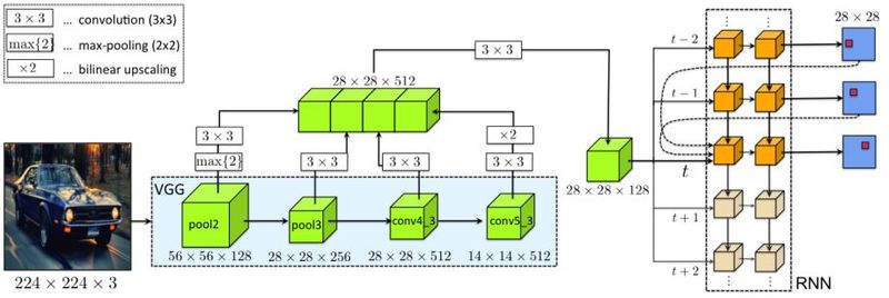
The authors have adopted the VGG16 feature extractor architecture with a few modifications pertaining to preservation of feature fused together in a tensor than can feed into the RNN (refer to Figure 2). Namely,the last max-pool layer present in the VGG16 CNN has been removed. The image fed into the CNN is pre-shrunk to a 224x224x3 tensor(3 being the Red, Green, and Blue channels). The image pass through 2 pooling layers with 128 and 2 convolutional layers. At each of these four steps, the idea is to have a width of 512 and so the output tensor at pool2 is convolved with 4 3x3x128 filters and the output tensor at pool3 is convolved with 2 3x3x256 filters. The skip connections from the four layers allows the CNN to extract low-level edge and corner features as well as boundary/semantic information about the instances.
