stat946w18/AmbientGAN: Generative Models from Lossy Measurements
Introduction
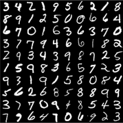
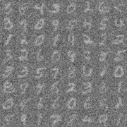
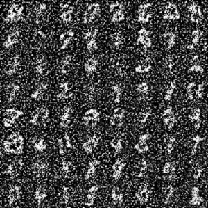
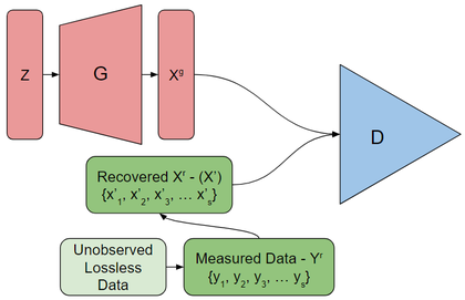
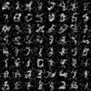
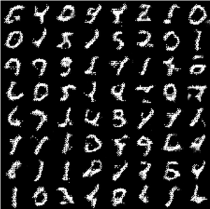
Generative models are powerful tools to concisely represent the structure in large datasets. Generative Adversarial Networks operate by simulating complex distributions but training them requires access to large amounts of high quality data. Often, we only have access to noisy or partial observations, which will, from here on, be referred to as measurements of the true data. If we know the measurement function and would like to train a generative model for the true data, there are several ways to continue which have varying degrees of success. We will use noisy MNIST data as an illustrative example, and show the results of 1. ignoring the problem, 2. trying to recover the lost information, and 3. using AmbientGAN as a way to recover the true data distribution. Suppose we only see MNIST data that has been run through a Gaussian kernel (blurred) with some noise from a [math]\displaystyle{ N(0, 0.5^2) }[/math] distribution added to each pixel:
-
True Data (Unobserved)
-
Measured Data (Observed)
Ignore the problem
Train a generative model directly on the measured data. This will obviously be unable to generate the true distribution before measurement has occurred.
Try to recover the information lost
Works better than ignoring the problem but depends on how easily the measurement function can be inverted.
AmbientGAN
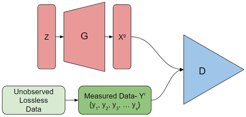
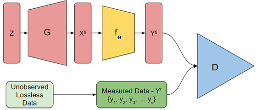
Ashish Bora, Eric Price and Alexandros G. Dimakis propose AmbientGAN as a way to recover the true underlying distribution from measurements of the true data. AmbientGAN works by training a generator which attempts to have the measurements of the output it generates fool the discriminator. The discriminator must distinguish between real and generated measurements. This paper is published in ICLR 2018.
Contributions
The paper makes the following contributions:
Theoretical Contribution
The authors show that the distribution of measured images uniquely determines the distribution of original images. This implies that a pure Nash equilibrium for the GAN game must find a generative model that matches the true distribution. They show similar results for a dropout measurement model, where each pixel is set to zero with some probability p, and a random projection measurement model, where they observe the inner product of the image with a random Gaussian vector.
Also, the author listed a few theorems to support assumptions satisfied under Gaussian-Projection, Convolve+Noise and Block-Pixels measurement models, thus showing that that we can recover the true underlying distribution with the AmbientGAN framework. For example, the Gaussian theorem guarantees the uniqueness of underlying distribution. Finally by showing that this assumption is satisfied under Gaussian-Projection, Convolve+Noise and Block-Pixels measurement models, the author finally proved that can recover the true underlying distribution with the AmbientGAN framework.
Empirical Contribution
The authors consider CelebA and MNIST dataset for which the measurement model is unknown and show that Ambient GAN recovers a lot of the underlying structure.
Related Work
Currently there exist two distinct approaches for constructing neural network based generative models; they are autoregressive [4,5] and adversarial [6] based methods. The adversarial model has shown to be very successful in modeling complex data distributions such as images, 3D models, state action distributions and many more. This paper is related to the work in [7] where the authors create 3D object shapes from a dataset of 2D projections. This paper states that the work in [7] is a special case of the AmbientGAN framework where the measurement process creates 2D projections using weighted sums of voxel occupancies.
Datasets and Model Architectures
We used three datasets for our experiments: MNIST, CelebA and CIFAR-10 datasets We briefly describe the generative models used for the experiments. For the MNIST dataset, we use two GAN models. The first model is a conditional DCGAN, while the second model is an unconditional Wasserstein GAN with gradient penalty (WGANGP). For the CelebA dataset, we use an unconditional DCGAN. For the CIFAR-10 dataset, we use an Auxiliary Classifier Wasserstein GAN with gradient penalty (ACWGANGP). For measurements with 2D outputs, i.e. Block-Pixels, Block-Patch, Keep-Patch, Extract-Patch, and Convolve+Noise, we use the same discriminator architectures as in the original work. For 1D projections, i.e. Pad-Rotate-Project, Pad-Rotate-Project-θ, we use fully connected discriminators. The architecture of the fully connected discriminator used for the MNIST dataset was 25-25-1 and for the CelebA dataset was 100-100-1.
Model
For the following variables superscript [math]\displaystyle{ r }[/math] represents the true distributions while superscript [math]\displaystyle{ g }[/math] represents the generated distributions. Let [math]\displaystyle{ x }[/math], represent the underlying space and [math]\displaystyle{ y }[/math] for the measurement.
Thus, [math]\displaystyle{ p_x^r }[/math] is the real underlying distribution over [math]\displaystyle{ \mathbb{R}^n }[/math] that we are interested in. However if we assume that our (known) measurement functions, [math]\displaystyle{ f_\theta: \mathbb{R}^n \to \mathbb{R}^m }[/math] are parameterized by [math]\displaystyle{ \Theta \sim p_\theta }[/math], we can then observe [math]\displaystyle{ Y = f_\theta(x) \sim p_y^r }[/math] where [math]\displaystyle{ p_y^r }[/math] is a distribution over the measurements [math]\displaystyle{ y }[/math].
Mirroring the standard GAN setup we let [math]\displaystyle{ Z \in \mathbb{R}^k, Z \sim p_z }[/math] and [math]\displaystyle{ \Theta \sim p_\theta }[/math] be random variables coming from a distribution that is easy to sample.
If we have a generator [math]\displaystyle{ G: \mathbb{R}^k \to \mathbb{R}^n }[/math] then we can generate [math]\displaystyle{ X^g = G(Z) }[/math] which has distribution [math]\displaystyle{ p_x^g }[/math] a measurement [math]\displaystyle{ Y^g = f_\Theta(G(Z)) }[/math] which has distribution [math]\displaystyle{ p_y^g }[/math].
Unfortunately, we do not observe any [math]\displaystyle{ X^g \sim p_x }[/math] so we cannot use the discriminator directly on [math]\displaystyle{ G(Z) }[/math] to train the generator. Instead we will use the discriminator to distinguish between the [math]\displaystyle{ Y^g - f_\Theta(G(Z)) }[/math] and [math]\displaystyle{ Y^r }[/math]. That is, we train the discriminator, [math]\displaystyle{ D: \mathbb{R}^m \to \mathbb{R} }[/math] to detect if a measurement came from [math]\displaystyle{ p_y^r }[/math] or [math]\displaystyle{ p_y^g }[/math].
AmbientGAN has the objective function:
\begin{align} \min_G \max_D \mathbb{E}_{Y^r \sim p_y^r}[q(D(Y^r))] + \mathbb{E}_{Z \sim p_z, \Theta \sim p_\theta}[q(1 - D(f_\Theta(G(Z))))] \end{align}
where [math]\displaystyle{ q(.) }[/math] is the quality function; for the standard GAN [math]\displaystyle{ q(x) = log(x) }[/math] and for Wasserstein GAN [math]\displaystyle{ q(x) = x }[/math].
As a technical limitation we require [math]\displaystyle{ f_\theta }[/math] to be differentiable with respect to each input for all values of [math]\displaystyle{ \theta }[/math].
With this set up we sample [math]\displaystyle{ Z \sim p_z }[/math], [math]\displaystyle{ \Theta \sim p_\theta }[/math], and [math]\displaystyle{ Y^r \sim U\{y_1, \cdots, y_s\} }[/math] each iteration and use them to compute the stochastic gradients of the objective function. We alternate between updating [math]\displaystyle{ G }[/math] and updating [math]\displaystyle{ D }[/math].
Measurement Models
The author consider the following model for measurement:
\textbf{Block-Pixels}Each pixel is independently set to zero with probability p.
Empirical Results
The paper continues to present results of AmbientGAN under various measurement functions when compared to baseline models. We have already seen one example in the introduction: a comparison of AmbientGAN in the Convolve + Noise Measurement case compared to the ignore-baseline, and the unmeasure-baseline.
Convolve + Noise
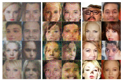
Additional results with the convolve + noise case with the celebA dataset. The AmbientGAN is compared to the baseline results with Wiener deconvolution. It is clear that AmbientGAN has superior performance in this case. The measurement is created using a Gaussian kernel and IID Gaussian noise, with [math]\displaystyle{ f_{\Theta}(x) = k*x + \Theta }[/math], where [math]\displaystyle{ * }[/math] is the convolution operation, [math]\displaystyle{ k }[/math] is the convolution kernel, and [math]\displaystyle{ \Theta \sim p_{\theta} }[/math] is the noise distribution.
Images undergone convolve + noise transformations (left). Results with Wiener deconvolution (middle). Results with AmbientGAN (right).
Block-Pixels
With the block-pixels measurement function each pixel is independently set to 0 with probability [math]\displaystyle{ p }[/math].
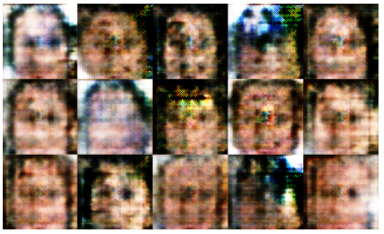
Measurements from the celebA dataset with [math]\displaystyle{ p=0.95 }[/math] (left). Images generated from GAN trained on unmeasured (via blurring) data (middle). Results generated from AmbientGAN (right).
Block-Patch
A random 14x14 patch is set to zero (left). Unmeasured using-navier-stoke inpainting (middle). AmbientGAN (right).
Pad-Rotate-Project-[math]\displaystyle{ \theta }[/math]
Results generated by AmbientGAN where the measurement function 0 pads the images, rotates it by [math]\displaystyle{ \theta }[/math], and projects it on to the x axis. For each measurement the value of [math]\displaystyle{ \theta }[/math] is known.
The generated images only have the basic features of a face and is referred to as a failure case in the paper. However the measurement function performs relatively well given how lossy the measurement function is.
For the Keep-Patch measurement model, no pixels outside a box are known and thus inpainting methods are not suitable. For the Pad-Rotate-Project-θ measurements, a conventional technique is to sample many angles, and use techniques for inverting the Radon transform . However, since only a few projections are observed at a time, these methods aren’t readily applicable hence it is unclear how to obtain an approximate inverse function shown below.
Explanation of Inception Score
To evaluate GAN performance, the authors make use of the inception score, a metric introduced by Salimans et al.(2016). To evaluate the inception score on a datapoint, a pre-trained inception classification model (Szegedy et al. 2016) is applied to that datapoint, and the KL divergence between its label distribution conditional on the datapoint and its marginal label distribution is computed. This KL divergence is the inception score. The idea is that meaningful images should be recognized by the inception model as belonging to some class, and so the conditional distribution should have low entropy, while the model should produce a variety of images, so the marginal should have high entropy. Thus an effective GAN should have a high inception score.
MNIST Inception
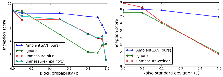
AmbientGAN was compared with baselines through training several models with different probability [math]\displaystyle{ p }[/math] of blocking pixels. The plot on the left shows that the inception scores change as the block probability [math]\displaystyle{ p }[/math] changes. All four models are similar when no pixels are blocked [math]\displaystyle{ (p=0) }[/math]. By the increase of the blocking probability, AmbientGAN models present a relatively stable performance and perform better than the baseline models. Therefore, AmbientGAN is more robust than all other baseline models.
The plot on the right reveals the changes in inception scores while the standard deviation of the additive Gaussian noise increased. Baselines perform better when the noise is small. By the increase of the variance, AmbientGAN models present a much better performance compare to the baseline models. Further AmbientGAN retains high inception scores as measurements become more and more lossy.
For 1D projection, Pad-Rotate-Project model achieved an inception score of 4.18. Pad-Rotate-Project-θ model achieved an inception score of 8.12, which is close to the score of vanilla GAN 8.99.
CIFAR-10 Inception
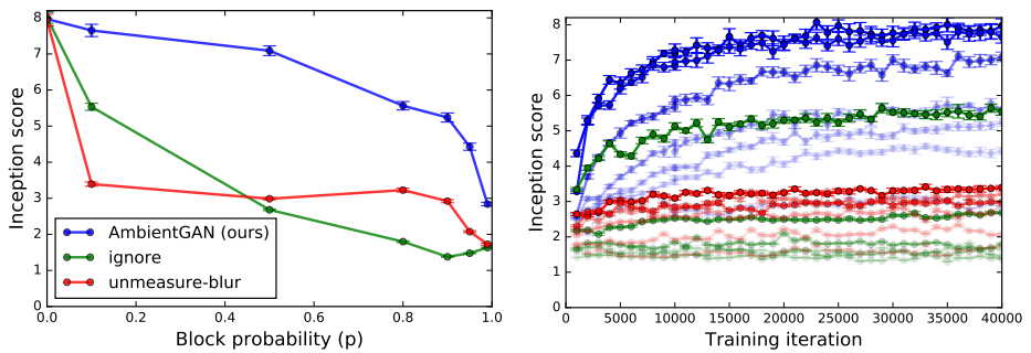
AmbientGAN is faster to train and more robust even on more complex distributions such as CIFAR-10. Similar trends were observed on the CIFAR-10 data, and AmbientGAN maintains relatively stable inception score as the block probability was increased.
Robustness To Measurement Model
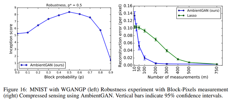
In order to empirically gauge robustness to measurement modelling error, the authors used the block-pixels measurement model: the image dataset was computed with [math]\displaystyle{ p^* = 0.5 }[/math], and several versions of the model were trained, each using different values of blocking probability [math]\displaystyle{ p }[/math]. The inception scores were calculated and plotted as a function of [math]\displaystyle{ p }[/math]. This is shown on the left below:
The authors observe that the inception score peaks when the model uses the correct probability, but decreases smoothly as the probability moves away, demonstrating some robustness.
Compressed Sensing
As described in Bora et al. (2017), generative models were found to outperform sparsity-based approaches in sensing. Using this knowledge, the generator from AmbientGAN can be tested against Lasso to determine the required measurements to minimize the reconstruction error. As shown on the right of Figure 16, AmbientGAN outperforms Lasso in a fraction of the number of measurements
Theoretical Results
The theoretical results in the paper prove the true underlying distribution of [math]\displaystyle{ p_x^r }[/math] can be recovered when we have data that comes from the Gaussian-Projection measurement, Fourier transform measurement and the block-pixels measurement. The do this by showing the distribution of the measurements [math]\displaystyle{ p_y^r }[/math] corresponds to a unique distribution [math]\displaystyle{ p_x^r }[/math]. Thus even when the measurement itself is non-invertible the effect of the measurement on the distribution [math]\displaystyle{ p_x^r }[/math] is invertible. Lemma 5.1 ensures this is sufficient to provide the AmbientGAN training process with a consistency guarantee. For full proofs of the results please see appendix A.
Lemma 5.1
Let [math]\displaystyle{ p_x^r }[/math] be the true data distribution, and [math]\displaystyle{ p_\theta }[/math] be the distributions over the parameters of the measurement function. Let [math]\displaystyle{ p_y^r }[/math] be the induced measurement distribution.
Assume for [math]\displaystyle{ p_\theta }[/math] there is a unique probability distribution [math]\displaystyle{ p_x^r }[/math] that induces [math]\displaystyle{ p_y^r }[/math].
Then for the standard GAN model if the discriminator [math]\displaystyle{ D }[/math] is optimal such that [math]\displaystyle{ D(\cdot) = \frac{p_y^r(\cdot)}{p_y^r(\cdot) + p_y^g(\cdot)} }[/math], then a generator [math]\displaystyle{ G }[/math] is optimal if and only if [math]\displaystyle{ p_x^g = p_x^r }[/math].
Theorems 5.2
For the Gussian-Projection measurement model, there is a unique underlying distribution [math]\displaystyle{ p_x^{r} }[/math] that can induce the observed measurement distribution [math]\displaystyle{ p_y^{r} }[/math].
Theorems 5.3
Let [math]\displaystyle{ \mathcal{F} (\cdot) }[/math] denote the Fourier transform and let [math]\displaystyle{ supp (\cdot) }[/math] be the support of a function. Consider the Convolve+Noise measurement model with the convolution kernel [math]\displaystyle{ k }[/math]and additive noise distribution [math]\displaystyle{ p_\theta }[/math]. If [math]\displaystyle{ supp( \mathcal{F} (k))^{c}=\phi }[/math] and [math]\displaystyle{ supp( \mathcal{F} (p_\theta))^{c}=\phi }[/math], then there is a unique distribution [math]\displaystyle{ p_x^{r} }[/math] that can induce the measurement distribution [math]\displaystyle{ p_y^{r} }[/math].
Theorems 5.4
Assume that each image pixel takes values in a finite set P. Thus [math]\displaystyle{ x \in P^n \subset \mathbb{R}^{n} }[/math]. Assume [math]\displaystyle{ 0 \in P }[/math], and consider the Block-Pixels measurement model with [math]\displaystyle{ p }[/math] being the probability of blocking a pixel. If [math]\displaystyle{ p \lt 1 }[/math], then there is a unique distribution [math]\displaystyle{ p_x^{r} }[/math] that can induce the measurement distribution [math]\displaystyle{ p_y^{r} }[/math]. Further, for any [math]\displaystyle{ \epsilon \gt 0, \delta \in (0, 1] }[/math], given a dataset of \begin{equation} s=\Omega \left( \frac{|P|^{2n}}{(1-p)^{2n} \epsilon^{2}} log \left( \frac{|P|^{n}}{\delta} \right) \right) \end{equation} IID measurement samples from pry , if the discriminator D is optimal, then with probability [math]\displaystyle{ \geq 1 - \delta }[/math] over the dataset, any optimal generator G must satisfy [math]\displaystyle{ d_{TV} \left( p^g_x , p^r_x \right) \leq \epsilon }[/math], where [math]\displaystyle{ d_{TV} \left( \cdot, \cdot \right) }[/math] is the total variation distance.
Conclusion
Generative models are powerful tools, but constructing a generative model requires a large, high quality dataset of the distribution of interest. The authors show how to relax this requirement, by learning a distribution from a dataset that only contains incomplete, noisy measurements of the distribution. This allows for the construction of new generative models of distributions for which no high quality dataset exists.
Future Research
One critical weakness of AmbientGAN is the assumption that the measurement model is known and that this [math]\displaystyle{ f_theta }[/math] is also differentiable. In fact, when the measurement model is known, there's no obvious reason not to invert the noisy measurement first(as illustrated in the second approach). It would be nice to be able to train an AmbientGAN model when we have an unknown measurement model but also a small sample of unmeasured data, or at the very least to remove the differentiability restriction from [math]\displaystyle{ f_theta }[/math].
A related piece of work is here. In particular, Algorithm 2 in the paper excluding the discriminator is similar to AmbientGAN.
Open Source Code
An implementation of Ambient GAN can be found here: https://github.com/AshishBora/ambient-gan.
References
- https://openreview.net/forum?id=Hy7fDog0b
- Salimans, Tim, et al. "Improved techniques for training gans." Advances in Neural Information Processing Systems. 2016.
- Szegedy, Christian, et al. "Rethinking the inception architecture for computer vision." Proceedings of the IEEE Conference on Computer Vision and Pattern Recognition. 2016.
- Diederik P Kingma and Max Welling. Auto-encoding variational bayes. arXiv:1312.6114, 2013.
- Aaron van den Oord, Sander Dieleman, Heiga Zen, Karen Simonyan, Oriol Vinyals, Alex Graves, Nal Kalchbrenner, Andrew Senior, and Koray Kavukcuoglu. Wavenet: A generative model for raw audio. arXiv preprint arXiv:1609.03499, 2016a.
- Ian Goodfellow, Jean Pouget-Abadie, Mehdi Mirza, Bing Xu, David Warde-Farley, Sherjil Ozair, Aaron Courville, and Yoshua Bengio. Generative adversarial nets. In Advances in neural infor- mation processing systems, pp. 2672–2680, 2014.
- Matheus Gadelha, Subhransu Maji, and Rui Wang. 3d shape induction from 2d views of multiple objects. arXiv preprint arXiv:1612.05872, 2016.
- Ashish Bora, Ajil Jalal, Eric Price, and Alexandros G Dimakis. Compressed sensing using generative models. arXiv preprint arXiv:1703.03208, 2017.
