stat946w18/IMPROVING GANS USING OPTIMAL TRANSPORT

Introduction

Generative Adversarial Networks (GANs) are powerful generative models. A GAN model consists of a generator and a discriminator or critic. The generator is a neural network which is trained to generate data having a distribution matched with the distribution of the real data. The critic is also a neural network, which is trained to separate the generated data from the real data. A loss function that measures the distribution distance between the generated data and the real one is important to train the generator.

Optimal transport theory evaluates the distribution distance based on metric, which provides another method for generator training. The main advantage of optimal transport theory over the distance measurement in GAN is its closed form solution for having a tractable training process. But the theory might also result in inconsistency in statistical estimation due to the given biased gradients if the mini-batches method is applied.

This paper presents a variant GANs named OT-GAN, which incorporates a discriminative metric called 'MIni-batch Energy Distance' into its critic in order to overcome the issue of biased gradients.

GANs and Optimal Transport

Generative Adversarial Nets

Original GAN was firstly reviewed. The objective function of the GAN:

The goal of GANs is to train the generator g and the discriminator d finding a pair of (g,d) to achieve Nash equilibrium. However, it could cause failure of converging since the generator and the discriminator are trained based on gradient descent techniques.

Wasserstein Distance (Earth-Mover Distance)

In order to solve the problem of convergence failure, Arjovsky et. al. (2017) suggested Wasserstein distance (Earth-Mover distance) based on the optimal transport theory.

where [math]\displaystyle{ \prod (p,g) }[/math] is the set of all joint distributions [math]\displaystyle{ \gamma (x,y) }[/math] with marginals [math]\displaystyle{ p(x) }[/math] (real data), [math]\displaystyle{ g(y) }[/math] (generated data). [math]\displaystyle{ c(x,y) }[/math] is a cost function and the Euclidean distance was used by Arjovsky et. al. in the paper.

The Wasserstein distance can be considered as moving the minimum amount of points between distribution [math]\displaystyle{ g(y) }[/math] and [math]\displaystyle{ p(x) }[/math] such that the generator distribution [math]\displaystyle{ g(y) }[/math] is similar to the real data distribution [math]\displaystyle{ p(x) }[/math].

Consider that solving the Wasserstein distance is usually not possible, the proposed Wasserstein GAN (W-GAN) provides an estimated solution by switching the optimal transport problem into dual formulation using a set of 1-Lipschitz functions. A neural network can then be used to obtain an estimation.

W-GAN solves the unstable training process of original GAN and it can solve the optimal transport problem approximately, but it is still intractable.

???The training process becomes traceable and a fully connected multi-layer network is sufficient for the training. However, the calculation of the Wasserstein distance is still an approximation and we can not have a fine-optimized critic.

Sinklhorn Distance

Genevay et al. (2017) proposed to use the primal formulation of optimal transport instead of the dual formulation to generative modeling. They introduced Sinkhorn distance which is a smoothed generalization of the Wasserstein distance.

It introduced entropy restriction ([math]\displaystyle{ \beta }[/math]) to the joint distribution [math]\displaystyle{ \prod_{\beta} (p,g) }[/math]. This distance could be generalized to approximate the mini-batches of data [math]\displaystyle{ X ,Y }[/math] with [math]\displaystyle{ K }[/math] vectors of [math]\displaystyle{ x, y }[/math]. The [math]\displaystyle{ i, j }[/math] th entry of the cost matrix [math]\displaystyle{ C }[/math] can be interpreted as the cost it needs to transport the [math]\displaystyle{ x_i }[/math] in mini-batch X to the [math]\displaystyle{ y_i }[/math] in mini-batch [math]\displaystyle{ Y }[/math]. The resulting distance will be:

where [math]\displaystyle{ M }[/math] is a [math]\displaystyle{ K \times K }[/math] matrix, each row of [math]\displaystyle{ M }[/math] is a joint distribution of [math]\displaystyle{ \gamma (x,y) }[/math] with positive entries. The summmation of rows or columns of [math]\displaystyle{ M }[/math] is always equal to 1.

This mini-batch Sinkhorn distance is not only fully tractable but also capable of solving the instability problem of GANs. However, it is not a valid metric over probability distribution when taking the expectation of [math]\displaystyle{ \mathcal{W}_{c} }[/math] and the gradients are biased when the mini-batch size is fixed.

Energy Distance (Cramer Distance)

In order to solve the above problem, Bellemare et al. proposed Energy distance:

where [math]\displaystyle{ x, x' }[/math] and [math]\displaystyle{ y, y' }[/math] are independent samples from data distribution [math]\displaystyle{ p }[/math] and generator distribution [math]\displaystyle{ g }[/math], respectively. Based on the Energy distance, Cramer GAN is to minimize the ED distance metric when training the generator.

MINI-BATCH ENERGY DISTANCE

Salimans et al. (2016) mentioned that comparing to use distributions over individual images, mini-batch GAN is more powerful when use the distributions over mini-batches [math]\displaystyle{ g(X), p(X) }[/math]. The distance measure is generated for mini-batches.

GENERALIZED ENERGY DISTANCE

The generalized energy distance allowed to use non-Euclidean distance functions d. It is also valid for mini-batches and is considered better than working with individual data batch.

Similarly as defined in the Energy distance, [math]\displaystyle{ X, X' }[/math] and [math]\displaystyle{ Y, Y' }[/math] can be the independent samples from data distribution [math]\displaystyle{ p }[/math] and the generator distribution [math]\displaystyle{ g }[/math], respectively. While in Generalized engergy distance, [math]\displaystyle{ X, X' }[/math] and [math]\displaystyle{ Y, Y' }[/math] can also be valid for mini-batches. The [math]\displaystyle{ D_{GED}(p,g) }[/math] is a metric when having [math]\displaystyle{ d }[/math] as a metric. Thus, taking the triangle inequality of [math]\displaystyle{ d }[/math] into account, [math]\displaystyle{ D(p,g) \geq 0, }[/math] and [math]\displaystyle{ D(p,g)=0 }[/math] when [math]\displaystyle{ p=g }[/math].

MINI-BATCH ENERGY DISTANCE

As [math]\displaystyle{ d }[/math] is free to choose, authors proposed Mini-batch Energy Distance by using entropy-regularized Wasserstein distnace as [math]\displaystyle{ d }[/math].

where [math]\displaystyle{ X, X' }[/math] and [math]\displaystyle{ Y, Y' }[/math] are independent sampled mini-batches from the data distribution [math]\displaystyle{ p }[/math] and the generator distribution [math]\displaystyle{ g }[/math], respectively. This distance metric combines the energy distance with primal form of optimal tranport over mini-batch distributions [math]\displaystyle{ g(Y) }[/math] and [math]\displaystyle{ p(X) }[/math]. Inside the generalized energy distance, the Sinkhorn distance is a valid metric between each mini-batches. By adding the [math]\displaystyle{ - \mathcal{W}_c (Y,Y') }[/math] and [math]\displaystyle{ \mathcal{W}_c (X,Y) }[/math] to equation (5) and using enregy distance, the objective becomes statistically consistent and mini-batch gradients are unbiased.

OPTIMAL TRANSPORT GAN (OT-GAN)

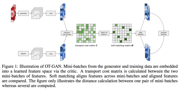
In order to secure the statistical efficiency, authors suggested using cosine distance between vectors [math]\displaystyle{ v_\eta (x) }[/math] and [math]\displaystyle{ v_\eta (y) }[/math] based on the deep neural network that maps the mini-batch data to a learned latent space. The reason for not using Euclidean distance is because of its poor performance in the high dimensional space. Here is the transportation cost:

where the [math]\displaystyle{ v_\eta }[/math] is chosen to maximize the resulting minibatch energy distance.

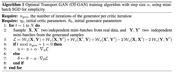
Unlike the practice when using the original GANs, the generator was trained more often than the critic, which keep the cost function from degeneration. The resulting generator in OT-GAN has a well defined and statistically consistent objective through the training process.

The algorithm is defined below. The backpropagation is not used in the algorithm due to the envelope theorem. Stochastic gradient descent is used as the optimization method.

EXPERIMENTS

In order to demonstrate the supermum performance of the OT-GAN, authors compared it with the original GAN and other popular models based on four experiments: Dataset recovery; CIFAR-10 test; ImageNet test; and the Conditional image synthesis test.

MIXTURE OF GAUSSIAN DATASET

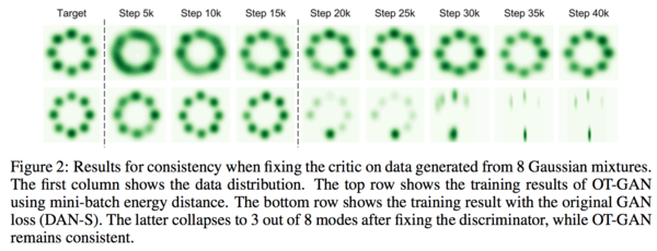
OT-GAN has a statistically consistent objective compare to the original GAN (DC-GAN), such that the generator would not update to a wrong direction even if the signal provided by the cost function to the generator is not good. In order to prove this advantage, authors compared the OT-GAN with the original GAN loss (DAN-S) based on a simple task. The task was set to recover all of the 8 modes from 8 Gaussian mixers in which the means were arranged in a circle. MLP with RLU activation functions were used in this task. The critic was only updated for 15K iterations. The generator distribution was tracked for another 25K iteration. The results showed that the original GAN experience the model collapse after fixing the discriminator while the OT-GAN recovered all the 8 modes from the mixed Gaussian data.

CIFAR-10

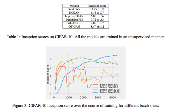
The dataset CIFAR-10 was then used for inspecting the effect of batch-size to the model training process and the image quality. OT-GAN and four other methods were compared using "inception score" as the criteria for comparison. Figure 3 shows the change of inceptions scores (y-axis) by the increased of the iteration number. Scores of four different batch sizes (200, 800, 3200 and 8000) were compared. The results show that a larger batch size would lead to a more stable model showing a larger value in inception score. However, a large batch size would also require a high-performance computational environment. The sample quality across all 5 methods are compared in Table 1 where the OT_GAN has the best score.

IMAGENET DOGS

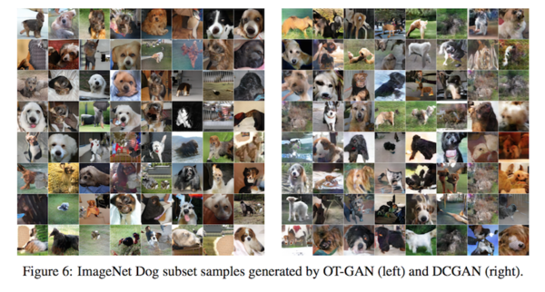
In order to investigate the performance of OT-GAN when dealing with the high-quality images, the dog subset of ImageNet (128*128) was used to train the model. Figure 6 shows that OT-GAN produces less nonsensical images and it has a higher inception score compare to the DC-GAN.

CONDITIONAL GENERATION OF BIRDS

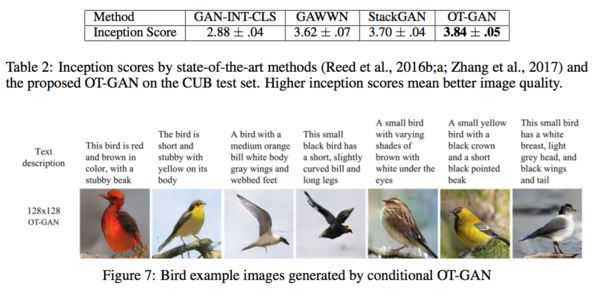
The last experiment was to compare OT-GAN with three popular GAN models for processing the text-to-image generation demonstrating the performance on conditional image synthesis. As can be found from Table 2, OT-GAN received the highest inception score than the scores of the other three models.

CONCLUSION

Authors presented a stable variant GAN named OT-GAN that the generator is trained through a newly defined distance metric, mini-batch energy distance, which is a combination of the primal form of the optimal transport and the energy distance. The mini-batch energy distance is a very discriminative distance function such that the metric still can give a correct direction when the critic is stop training or even the cost signal is very weak and it also has unbiased gradients. OT-GAN has outstanding performance compared to several other GANs when training with relatively large batch size. However, the large mini-batches requires high performance of computational environment and it is also very time consuming.

CRITIQUE

The paper presents a variant of GANs by defining a new distance metric which is combing the primal form of optimal transport and the mini-batch energy distance. The Gaussian toy example has proven that the OT-GAN has a very stable objective function since it remains valid when the discriminator stops training. The CIFAR-10 data example also proved that OT-GAN is very stable when large mini-batches are applied.

However, here still has some limitations. First of all, the authors mentioned that OT-GAN is a stable algorithm when the batch size is large. In the CIFAR-10 example, the algorithm has an outstanding performance when the batch size is 8000. This might lead to the computational inefficiency problem.

Furthermore, in section 2, the paper is lack of explanation about how the Sinkhorn distance changes from taking a vector as input to using the mini-batches as the input. It is quite confusing when they explain the algorithm in section 4 about how M is chosen to minimize [math]\displaystyle{ \mathcal{W} }[/math].