Deep Exploration via Bootstrapped DQN

Intro to Reinforcement Learning

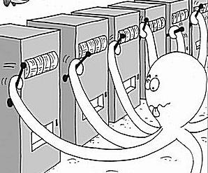
In reinforcement learning, an agent interacts with an environment with the goal to maximize its long term reward. A common application of reinforcement learning is to the multi armed bandit problem. In a multi armed bandit problem, there is a gambler and there are $n$ slot machines, and the gambler can choose to play any specific slot machine at any time. All the slot machines have their own probability distributions by which they churn out rewards, but this is unknown to the gambler. So the question is, how can the gambler learn how to get the maximum long term reward?

There are two things the gambler can do at any instance: either he can try a new slot machine, or he can play the slot machine he has tried before (and he knows he will get some reward). However, even though trying a new slot machine feels like it would bring less reward to the gambler, it is possible that the gambler finds out a new slot machine that gives a better reward than the current best slot machine. This is the dilemma of exploration vs exploitation. Trying out a new slot machine is exploration, while redoing the best move so far is exploiting the currently understood perception of the reward.

Source: blogs.mathworks.com

There are many strategies to approach this exploration-exploitation dilemma. A simple list of strategies can be found online here. A lot of these approaches are provably efficient, but assume that the state space is not very large. For instance, the approach called Curiosity-Driven Exploration is aiming at taking actions that lead to immediate additional information. This requires the model to search “every possible cell in the grid” which is not desirable if state space is very large. Strategies for large state spaces often just either ignore exploration, or do something naive like $\epsilon$-greedy, where you exploit with $1-\epsilon$ probability and explore "randomly" in rest of the cases.

This paper tries to use a Thompson sampling like approach to make decisions.

Thompson Sampling^[1]

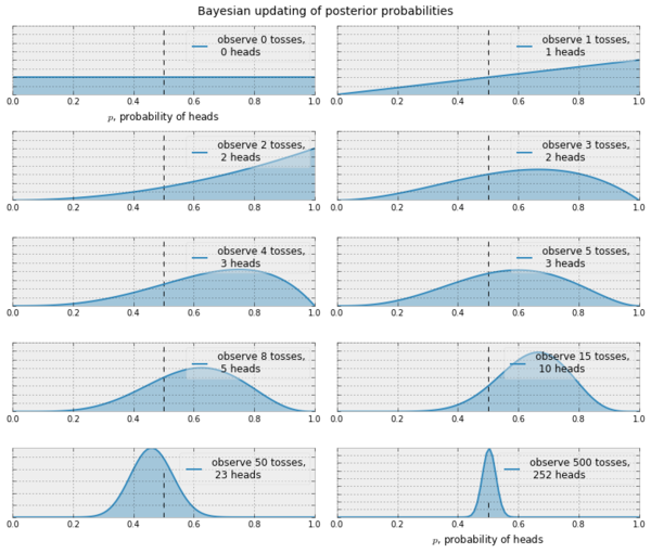
In Thompson sampling, our goal is to reach a belief that resembles the truth. Let's consider a case of coin tosses (2-armed bandit). Suppose we want to be able to reach a satisfactory pdf for $\mathbb{P}_h$ (heads). Assuming that this is a Bernoulli bandit problem, i.e. the rewards are $0$ or $1$, we can start off with $\mathbb{P}_h^{(0)}=\beta(1,1)$. The $\beta(x,y)$ distribution is a very good choice for a possible pdf because it works well for Bernoulli rewards. Further $\beta(1,1)$ is the uniform distribution $\mathbb{N}(0,1)$.

Now, at every iteration $t$, we observe the reward $R^{(t)}$ and try to make our belief close to the truth by doing a Bayesian computation. Assuming $p$ is the probability of getting a heads,

$$ \begin{align*} \mathbb{P}(R|D) &\propto \mathbb{P}(D|R) \cdot \mathbb{P}(R) \\ \mathbb{P}_h^{(t+1)}&\propto \mbox{likelihood}\cdot\mbox{prior} \\ &\propto p^{R^{(t)}}(1-p)^{R^{(t)}} \cdot \mathbb{P}_h^{(t)} \\ &\propto p^{R^{(t)}}(1-p)^{R^{(t)}} \cdot \beta(x_t, y_t) \\ &\propto p^{R^{(t)}}(1-p)^{R^{(t)}} \cdot p^{x_t-1}(1-p)^{y_t-1} \\ &\propto p^{x_t+R^{(t)}-1}(1-p)^{y_t+R^{(t)}-1} \\ &\propto \beta(x_t+R^{(t)}, y_t+R^{(t)}) \end{align*} $$

Source: Quora

This means that with successive sampling, our belief can become better at approximating the truth. There are similar update rules if we use a non Bernoulli setting, say, Gaussian. In the Gaussian case, we start with $\mathbb{P}_h^{(0)}=\mathbb{N}(0,1)$ and given that $\mathbb{P}_h^{(t)}\propto\mathbb{N}(\mu, \sigma)$ it is possible to show that the update rule looks like

$$ \mathbb{P}_h^{(t+1)} \propto \mathbb{N}\bigg(\frac{t\mu+R^{(t)}}{t+1},\frac{\sigma}{\sigma+1}\bigg) $$

How can we use this in reinforcement learning?

We can use this idea to decide when to explore and when to exploit. We start with an initial belief, choose an action, observe the reward and based on the kind of reward, we update our belief about what action to choose next.

Bootstrapping ^[2,3]

This idea may be unfamiliar to some people, so I thought it would be a good idea to include this. In statistics, bootstrapping is a method to generate new samples from a given sample. Suppose that we have a given population, and we want to study a measure $\theta$. So, we just find $n$ sample points (sample $\{D_i\}_{i=1}^n$), calculate this measure $\hat{\theta}$ for these $n$ points, and make our inference.

If we later wish to find a better bound on $\hat{\theta}$, i.e. suppose we want to say that $\delta_1 \leq \hat{\theta} \leq \delta_2$ with a confidence of $c$, then we can use bootstrapping for this.

Using bootstrapping, we can create a new sample $\{D'_i\}_{i=1}^{n'}$ by randomly sampling $n'$ times from $D$, with replacement. So, if $D=\{1,2,3,4\}$, a $D'$ of size $n'=10$ could be $\{1,4,4,3,2,2,2,1,3,4\}$. We do this a sufficient $k$ number of times, calculate $\hat{\theta}$ each time, and thus get a distribution $\{\hat{\theta}_i\}_{i=1}^k$. Now, we can choose the $100\cdot c$^th and $100\cdot(1-c)$^th percentile of this distribution, (let them be $\hat{\theta}_\alpha$ and $\hat{\theta}_\beta$ respectively) and say

$$\hat{\theta}_\alpha \leq \hat{\theta} \leq \hat{\theta}_\beta, \mbox{with confidence }c$$

Why choose bootstrap and not dropout?

There is previous work^[4] that establishes dropout as a good way to train NNs on a posterior such that the trained NN works like a function approximator that is close to the actual posterior. But, there are several problems with the predictions of this trained NN. The figures below are from the appendix of this paper. The left image is the NN trained by the authors of this paper on a sample noisy distribution and the right image is from the accompanying web demo from [4], where the authors of [4] show that their NN converges around the mean with a good confidence.

Source: this paper's appendix

According to the authors of this paper,

1. Even though [4] says that dropout converges arond the mean, their experiment actually behaves weirdly around a reasonable point like $x=0.75$. They think that this happens because dropout only affects the region local to the original data.
2. Samples from the NN trained on the original data do not look like a reasonable posterior (very spiky).
3. The trained NN collapses to zero uncertainty at the data points from the original data.

References

1. Learning and optimization for sequential decision making, Columbia University, Lec 4
2. Thoughtco, What is bootstrapping in statistics?
3. Bootstrap confidence intervals, Class 24, 18.05, MIT Open Courseware
4. Yarin Gal and Zoubin Ghahramani. Dropout as a bayesian approximation: Representing model uncertainty in deep learning. arXiv preprint arXiv:1506.02142, 2015.