STAT946F17/ Coupled GAN

This is a summary of NIPS 2016 paper [1].

Introduction

Generative models attempt to characterize and estimate the underlying probability distribution of the data (typically images) and in doing so generate samples from the aforementioned learned distribution. Moment-matching generative networks, Variational auto-encoders, and Generative Adversarial Networks (GANs) are some of the most popular (and recent) class of techniques in this burgeoning literature on generative models. The authors of the paper we are reviewing focus on proposing an extension to the class of GANs.

The novelty of the proposed Coupled GAN (CoGAN) method lies in extending the GAN procedure (described in the next section) to the multi-domain setting. That is, the CoGAN methodology attempts to learn the (underlying) joint probability distribution of multi-domain images as a natural extension from the marginal setting associated with the vanilla GAN framework. This is inspired by the idea that deep neural networks learn a hierarchical feature representation. Given the dense and active literature on generative models, generating images in multiple domains is far from groundbreaking. Related works revolve around multi-modal deep learning ([2],[3]), semi-coupled dictionary learning ([4]), joint embedding space learning ([5]), cross-domain image generation ([6],[7]) to name a few. Thus, the novelty of the authors' contributions to this field comes from two key differentiating points. Firstly, this was (one of) the first papers to endeavor to generate multi-domain images with the GAN framework. Secondly, and perhaps more significantly, the authors proposed to learn the underlying joint distribution without requiring the presence of tuples of corresponding images in the training set. Only sets of images drawn from the (marginal) distributions of the separate domains is sufficient. As per the authors' claim, constructing tuples of corresponding images to train from is challenging and a potential bottleneck for multi-domain image generation. One way around this bottleneck is thus to use their proposed CoGAN methodology. More details of how the authors achieve joint-distribution learning will be provided in the Coupled GAN section below.

Generative Adversarial Networks

A typical GAN framework consists of a generative model and a discriminative model. The generative model, which often is a de-convolutional network, takes as input a random latent vector (typically uniform or Gaussian) and synthesizes novel images resembling the real images (training set). The discriminative model, often a convolutional network, on the other hand, tries to distinguish between the fake synthesized images and the real images. The idea then is to let the two component models of the GAN framework "compete" with each other in the form of a min-max two player game.

To further clarify and fix this idea, we introduce the mathematical setup of GANs following the notation used by the authors of this paper for sake of consistency. Let us define the following in our setup:

[math]\displaystyle{ \mathbf{x}- }[/math] natural image drawn from underlying distribution [math]\displaystyle{ p_X }[/math],

[math]\displaystyle{ \mathbf{z} \sim U[-1,1]^d- }[/math] a latent random vector,

$g-$ generative model, $f-$ discriminative model.

Ideally we are aiming for the system of these two adversarial networks to behave as:

Generator: $g(\mathbf{z})$ outputs an image with same support as $\mathbf{x}$. The probability density of the images output by $g$ can be denoted by $p_G$,

Discriminator: $f(\mathbf{x})=1$ if $\mathbf{x} \sim p_X$ and $f(\mathbf{x})=0$ if $\mathbf{x} \sim p_G$.

To train such a system of networks given our goal (i.e., $p_G \rightarrow p_X$) we must treat such a framework as the following minimax two player game:

$\displaystyle \max_{g}$ $\min\limits_{f} V(g,f) = \mathop{\mathbb{E}}_{\mathbf{x} \sim p_X}[-\log(f(\mathbf{x}))] + \mathop{\mathbb{E}}_{\mathbf{z} \sim p_{Z}(\mathbf{z})}[-\log(1-f(g(\mathbf{z})))] $.

See [8], the seminal paper on this topic, for more information.

Some of the crucial advantages of GANs are that Markov chains are never needed, only backprop is used to obtain gradients, no inference is needed during learning, and a wide variety of functions can be incorporated into the model [16].

Coupled Generative Adversarial Networks

The overarching goal of this framework is to learn a joint distribution of multi-domain images from data. That is, a density value is assigned to each joint occurrence of images in different domains. Examples of such pair of images in different domains include images of a particular scene with different modalities (color and depth) or images of the same face but with different facial attributes.

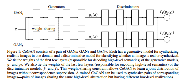
To this end, the CoGAN setup consists of a pair of GANs, denoted as $GAN_1$ and $GAN_2$. Each GAN is tasked with synthesizing images in one domain. A naive training of such a system will result in learning the product of the two marginal distributions i.e., independence. However, by forcing the two GANs to share weights, the authors were able to demonstrate that they could in some sense learn the joint distribution of images. We will now describe the details of the generator and discriminator components of the setup and conclude this section with a summary of CoGAN learning algorithm.

Generator Models

Suppose $\mathbf{x_1} \sim p_{X_1}$ and $\mathbf{x_2} \sim p_{X_2}$ denote the natural images being drawn from the two marginal distributions of domain 1 and domain 2. Further, let $g_1$ be the generator of $GAN_1$ and $g_2$ be the generator of $GAN_2$. Both these generators take as input the latent vector $\mathbf{z}$ as defined in the previous section as input and out images in their specific domains. For completeness, denote the distributions of $g_1(\mathbf{z})$ and $g_2(\mathbf{z})$ as $p_{G_1}$ and $p_{G_2}$ respectively. We can characterize these two generator models as multi-layer perceptrons in the following way:

\begin{align*} g_1(\mathbf{z})=g_1^{(m_1)}(g_1^{(m_1 -1)}(\dots g_1^{(2)}(g_1^{(1)}(\mathbf{z})))), \quad g_2(\mathbf{z})=g_2^{(m_2)}(g_2^{(m_2-1)}(\dots g_2^{(2)}(g_2^{(1)}(\mathbf{z})))), \end{align*} where $g_1^{(i)}$ and $g_2^{(i)}$ are the $i^{th}$ layers of $g_1$ and $g_2$ which respectively have a total of $m_1$ and $m_2$ layers each. Note $m_1$ need not be the same as $m_2$.

As the generator networks can be thought of as an inverse of the prototypical convolutional networks (just as an example), the layers of these generator networks gradually decode information from high-level abstract concepts to low-level details(last few layers). Taking this idea as the blueprint for the inner-workings of generator networks, the author's hypothesize that corresponding images in two domains share the same high-level semantics but with differing lower-level details. To put this hypothesis to practice, they forced the first $k$ layers of $g_1$ and $g_2$ to have identical structures and share the same weights. That is, $\mathbf{\theta}_{g_1^{(i)}}=\mathbf{\theta}_{g_2^{(i)}}$ for $i=1,\dots,k$ where $\mathbf{\theta}_{g_1^{(i)}}$ and $\mathbf{\theta}_{g_1^{(i)}}$ represents the parameters of the layers $g_1^{(i)}$ and $g_2^{(i)}$ respectively. Hence the two generator networks share the starting $k$ layers of the deep network and have different last layers to decode the differing material details in each domain.

Discriminative Models

Suppose $f_1$ and $f_2$ are the respective discriminative models of the two GANs. These models can be characterized by \begin{align*} f_1(\mathbf{x}_1)=f_1^{(n_1)}(f_1^{(n_1 -1)}(\dots f_1^{(2)}(f_1^{(1)}(\mathbf{x}_1)))), \quad f_2(\mathbf{x}_2)=f_2^{(n_2)}(f_2^{(n_2-1)}(\dots f_2^{(2)}(f_2^{(1)}(\mathbf{x}_1)))), \end{align*} where $f_1^{(i)}$ and $f_2^{(i)}$ are the $i^{th}$ layers of $f_1$ and $f_2$ which respectively have a total of $n_1$ and $n_2$ layers each. Note $n_1$ need not be the same as $n_2$. In contrast to generator models, the first layers of $f_1$ and $f_2$ extract the lower level details where the last layers extract the abstract higher level details. To reflect the prior hypothesis of shared higher level semantics between corresponding images, we can force $f_1$ and $f_2$ to now share the weights for last $l$ layers. That is, $\mathbf{\theta}_{f_1^{(n_1-i)}}=\mathbf{\theta}_{f_2^{(n_2-i)}}$ for $i=0,\dots,l-1$ where $\mathbf{\theta}_{f_1^{(i)}}$ and $\mathbf{\theta}_{f_1^{(i)}}$ represents the parameters of the layers $f_1^{(i)}$ and $f_2^{(i)}$ respectively. Unlike in the generative models, weight sharing in the discriminative models is not essential to estimating the joint distribution of images, however it is beneficial by reducing the total number of parameters in the network.

Coupled GAN (CoGAN) Framework and Learning

The following figure taken from the paper summarizes the system of models described in the previous subsections.

The CoGAN framework can be expressed as the following constrained min-max game

\begin{align*} \max\limits_{g_1,g_2} \min\limits_{f_1, f_2} V(f_1,f_2,g_1,g_2)\quad \text{subject to} \ \mathbf{\theta}_{g_1^{(i)}}=\mathbf{\theta}_{g_2^{(i)}}, i=1,\dots k, \quad \mathbf{\theta}_{f_1^{(n_1-j)}}=\mathbf{\theta}_{f_2^{(n_2-j)}}, j=1,\dots,l-1, \end{align*} where the value function V is characterized as \begin{align*} \mathop{\mathbb{E}}_{\mathbf{x}_1 \sim p_{X_1}}[-\log(f_1(\mathbf{x_1}))] + \mathop{\mathbb{E}}_{\mathbf{z} \sim p_{Z}(\mathbf{z})}[-\log(1-f_1(g_1(\mathbf{z})))]+\mathop{\mathbb{E}}_{\mathbf{x}_2 \sim p_{X_2}}[-\log(f_2(\mathbf{\mathbf{x}_2}))] + \mathop{\mathbb{E}}_{\mathbf{z} \sim p_{Z}(\mathbf{z})}[-\log(1-f_2(g_2(\mathbf{z})))]. \end{align*}

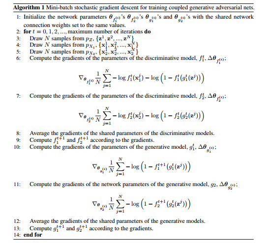
For the purposes of storytelling, we can describe this game to have two teams with two players each. The generative models are in the same team and collaborate with each other to synthesize a pair of images in two different domains with goal of fooling the discriminative models. The discriminative models than with collaboration try to differentiate between images drawn from the training data in their respective domains and the images generated by the respective generative models. The training algorithm for the CoGAN that was used is described in the following figure.

Important Remarks:

CoGAN learning requires training samples drawn from the marginal distributions, $p_{X_1}$ and $p_{X_2}$ . It does not rely on samples drawn from the joint distribution, $p_{X_1,X_2}$ , where corresponding supervision would be available. Here, the main contribution is in showing that with just samples drawn separately from the marginal distributions, CoGAN can learn a joint distribution of images in the two domains. Both weight-sharing constraint and adversarial training are essential for enabling this capability.

Unlike autoencoder learning which encourages the generated image pair to be identical to the target pair , the adversarial training only encourages the generated pair of images to be individually resembling the images in the respective domains, and ignore the correlation between them. Shared parameters, on the other hand, contribute to matching the correlation: the neurons responsible for decoding high-level semantics can be shared to produce highly correlated image pairs.

Experiments

To begin with, note that the authors do not use corresponding images in the training set in accordance with the goal of learning the joint distribution of multi-domain images without correspondence supervision. As at the time the paper was written, there were no existing approached with identical prerogatives (i.e., training with no correspondence supervision), they compared CoGAN with conditional GAN (see [10]) for more details on conditional GAN).

MNIST Dataset

The MNIST training set was experimented with two tasks:

1. Task A: Learning a joint distribution of a digit and its edge image.
2. Task B: Learning a joint distribution of a digit and its negative image.

For the generative models, the authors used convolutional networks with 5 identical layers. They varied the number of shared layers as part of their experimental setup. The two discriminative models were a version of the LeNet ([9]). The results of the CoGAN generation scheme are displayed in the figure below.

As you can see from the figure above, the CoGAN system was able to generate pairs of corresponding images without explicitly training with correspondence supervision. This was naturally due to sharing weights in lower levels used for decoding high-level semantics. Without sharing these weights, the CoGAN would just output a pair of unrelated images in the two domains.

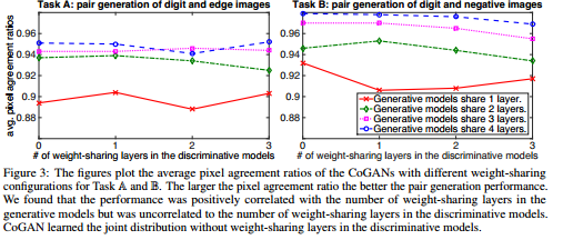
To investigate the effects of weight sharing in the generator/discriminator models used for both tasks, the authors varied the number of shared levels. To quantify the performance of the generator, the image generated by $GAN_1$ (domain 1) was transformed to the 2nd domain using the same method used to generate training images in the 2nd domain. Then this transformed image was compared with the image generated by $GAN_2$. Naturally, if the joint distribution was learned completely, these two images would be identical. With that goal in mind, the authors used pixel agreement ratios for 10000 images as the evaluation metric. In particular, 5 trails with different weight initializations were used and an average pixel agreement ratio was taken. The results depicting the relationship between the average pixel agreement ratio and a number of shared layers are summarized in the figure below.

The results naturally offered some corroboration to our intuitions. The greater the number of shared layers in the generator models, the higher the pixel agreement ratios. Interestingly the number of shared layers in the discriminative model does not seem to affect the pixel agreement ratios. Note this is a pretty naive and toy example as we by nature of the evaluation criteria have a deterministic way of generating an image in the 2nd domain.

Finally, for this example, the authors compared the CoGAN framework with the conditional GAN model. For the conditional GAN, the generative and discriminative models were identical to those used for the CoGAN results. The conditional GAN additionally took a binary variable (the conditioning variable) as input. When the binary variable was 0, the conditional GAN synthesized an image in domain 1 and when it was 1 an image in domain 2. Naturally, for a fair comparison, the training set did not already contain corresponding pairs of images. The experiments were conducted for the two tasks described above and the pixel agreement ratio (PAR) was the evaluation criteria. For Task A, the CoGAN resulted in a PAR of 0.952 in comparison with 0.909 for the conditional GAN. For Task B, the CoGAN resulted in a PAR of 0.967 compared with a PAR of 0.778 for the conditional GAN. The results are not particularly eye opening as the CoGAN was more specifically designed for purpose of learning the joint distribution of multi-domain images whereas these tasks are just a very niche application for the conditional GAN. Nevertheless, for Task B, the results look promising.

CelebFaces Attributes Dataset

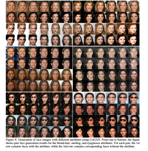
For this experiment, the authors trained the CoGAN, using the CelebFaces Attributes Dataset, to generate pairs of faces with an attribute (domain 1) and without the attribute (domain 2). CelebFaces Attributes Dataset (CelebA) is a large-scale face attributes dataset with more than 200K celebrity images, each with 40 attribute annotations. The images in this dataset cover large pose variations and background clutter. CelebA has large diversities, large quantities, and rich annotations, including 10,177 number of identities, 202,599 number of face images, and 5 landmark locations, 40 binary attributes annotations per image. Convolutional networks with 7 layers for both the generative and discriminative models were used. The dataset contains a large variety of poses and background clutter. Attributes can include blonde/non-blonde hair, smiling/ not smiling, or with/without sunglasses for example. The resulting synthesized pair of images are shown in the figure below realized as spectrum traveling from one point to another (resembles changing faces).

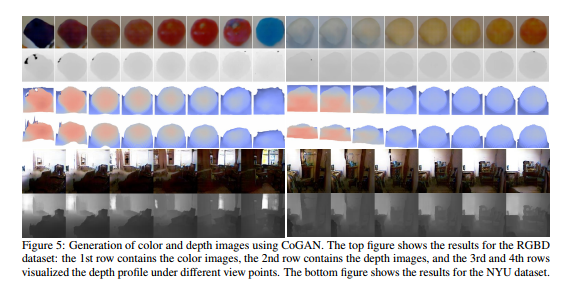
Color and Depth Images

For this experiment the authors used two sources: the RGBD dataset and the NYU dataset. The two image domains (color-domain 1 and depth-domain 2) under consideration are the same for both the datasets. As usual, no corresponding images were fed into the training of the CoGAN framework. The resulting rendering of pairs of color and depth images for both the datasets are depicted in the figure below.

As is evident from the images, through the sharing of layers during training, the CoGAN was able to learn the appearance-depth correspondence.

Applications

Unsupervised Domain Adaptation (UDA)

UDA involves adapting a classifier trained in one domain to conduct a classification task in a new domain which only contains unlabeled training data which disqualifies re-training of the classifier in this new domain. Some prior work in the field includes subspace learning ([11],[12]) and deep discriminative network learning ([13],[14]). The authors in the paper experimented with the MNIST and USPS datasets to showcase the applicability of the CoGAN framework for the UDA problem. A similar network architecture as was used for the MNIST experiment was employed for this application. The MNIST and USPS datasets has been denoted as $D_1$ and $D_2$ respectively in the paper. In accordance with the problem specification, no label information was used from $D_2$.

The CoGAN is trained by jointly solving the classification problem in the MNIST domain using the labels provided in $D_1$ and the CoGAN learning problem which uses images in both $D_1$ and $D_2$. This training process produces two classifiers. That is, $c_1(x_1)=c(f_1^{(3)}(f_1^{(2)}(f_1^{(1)}(x_1))))$ for MNIST and $c_2(x_2)=c(f_2^{(3)}(f_2^{(2)}(f_2^{(1)}(x_2))))$ and USPS. Note $c()$ here denotes the softmax layer which is added on top of the other layers in the respective discriminative networks of the GANs. Further due to weight sharing the last two layers of the discriminative model would be identical and have the same weights. The classifier $c_2$ is then used for digit classification in the USPS dataset. The author reported a 91.2% average accuracy when classifying the USPS dataset. The mirror problem of classifying the MNIST dataset without labels using the fully characterized USPS dataset achieved an average accuracy of 89.1%. These results appear to significantly outperform (prior top classification accuracy lies roughly around 60-65%) what the authors claim to be the state of the art methods in the UDA literature. In particular the state of the art was noted to be described in [20].

Cross-Domain Image Transformation

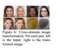
Let $\mathbf{x}_1$ be a image in the 1st domain. The goal then is to find a corresponding image $\mathbf{x}_2$ in 2nd domain such that the joint probability density $p(\mathbf{x}_1,\mathbf{x}_2)$ is maximized. Given the two generators $g_1$ and $g_2$, one can achieve the cross-domain transformation by first finding the latent random vector that generates the input image $\mathbf{x}_1$ in the 1st domain. This amounts to the optimization: $\mathbf{z}^{*}=argmin_{\mathbf{z}}L(g_1(\mathbf{z}),\mathbf{x}_1)$, where $L$ is the loss function measuring the difference/distance between the two images. After finding $z^*$, one can apply $g_2$ to obtain the transformed image, $x_2 = g_2(z^*)$. Some very preliminary results were are provided by the authors. Namely, the authors concluded that the transformation was successful when the input image was covered by $g_{1}$, but generated blurry images when this was not the case. Overall, there is nothing noteworthy to warrant discussion. It is hypothesized that more training images are required in addition to a better objective function. The figure depicting their results is provided below for sake of completeness.

Eyewitness Facial Composite Generation

Since a Coupled GAN requires only a small set of images acquired separately from the marginal distributions of the individual domains, forensic criminal feature generation could find use for CoGAN. Due to the high noise and variation in facial composites derived from eyewitness statements (marginal), CoGAN could assist in narrowing down the search space.

Live Criminal Identification

Given a sufficiently large data set of images of a criminal (marginal) and sufficiently large data set of the images of ubiquitous places (e.g, local store, grocery stores, streets etc) (destination marginal), it would be possible to feed live footage to the coupled GAN discriminators for identifying & timestamping criminal visited locations

Discussion and Summary

The main contributions of the paper can be summarized as:

1. A CoGAN framework for learning a joint distribution of multi-domain images was proposed.
2. The training is achieved by a simple weight sharing scheme for the generative and discriminative networks in the absence of any correspondence supervision in the training set. This can be construed as learning the joint distribution by using samples from the marginal distribution of images.
3. The experiments with digits, faces, and color/depth images provided some corroboration that the CoGAN system could synthesize corresponding pairs of images.
4. An application of the CoGAN framework for the problem of Unsupervised Domain Adaptation (UDA) was introduced. The preliminary results appear to be extremely promising for the task of adapting digit classifiers from MNIST to USPS data and vice-versa.
5. An application for the task of cross-domain image transformation was hypothesized with some very basic proof of concept results provided.
6. The setup naturally lends to more than the two domain setting focused on in the paper for experimental purposes.

While the summary provided above adopted an objective filter, the following list enumerates the major subjective critical review points for this paper:

1. It appears the authors took components of various well-established techniques in the literature and produced the CoGAN framework. Weight-sharing is a well documented idea as was correspondance/ multi-modal learning along with the GAN problem formation and training. However, when the components are put together in this way, they form a modest and timely novel contribution to the literature of generative networks.
2. With such prominent preliminary results for the problem of UDA, the authors could have provided some additional details of their training procedure (slightly unclear) and additional experiments under the UDA umbrella to fortify what appears to be a ground breaking result when compared with state of the art methods.
3. The cross-domain image transformation application example was almost an after thought. More details could have been provided in the supplementary file if pressed for space or perhaps just merely relegated to a follow-up paper/work.

References and Supplementary Resources

[1] Liu, Ming-Yu, and Oncel Tuzel. "Coupled generative adversarial networks." Advances in neural information processing systems. 2016.

[2] Srivastava, Nitish, and Ruslan R. Salakhutdinov. "Multimodal learning with deep boltzmann machines." Advances in neural information processing systems. 2012.

[3] Ngiam, Jiquan, et al. "Multimodal deep learning." Proceedings of the 28th international conference on machine learning (ICML-11). 2011.

[4] Wang, Shenlong, et al. "Semi-coupled dictionary learning with applications to image super-resolution and photo-sketch synthesis." Computer Vision and Pattern Recognition (CVPR), 2012 IEEE Conference on. IEEE, 2012.

[5] Kiros, Ryan, Ruslan Salakhutdinov, and Richard S. Zemel. "Unifying visual-semantic embeddings with multimodal neural language models." arXiv preprint arXiv:1411.2539 (2014).

[6] Yim, Junho, et al. "Rotating your face using multi-task deep neural network." Proceedings of the IEEE Conference on Computer Vision and Pattern Recognition. 2015.

[7] Reed, Scott E., et al. "Deep visual analogy-making." Advances in neural information processing systems. 2015.

[8] Goodfellow, Ian, et al. "Generative adversarial nets." Advances in neural information processing systems. 2014.

[9] LeCun, Yann, et al. "Gradient-based learning applied to document recognition." Proceedings of the IEEE 86.11 (1998): 2278-2324.

[10] Mirza, Mehdi, and Simon Osindero. "Conditional generative adversarial nets." arXiv preprint arXiv:1411.1784 (2014).

[11] Long, Mingsheng, et al. "Transfer feature learning with joint distribution adaptation." Proceedings of the IEEE international conference on computer vision. 2013.

[12] Fernando, Basura, Tatiana Tommasi, and Tinne Tuytelaars. "Joint cross-domain classification and subspace learning for unsupervised adaptation." Pattern Recognition Letters 65 (2015): 60-66.

[13] Tzeng, Eric, et al. "Deep domain confusion: Maximizing for domain invariance." arXiv preprint arXiv:1412.3474 (2014).

[14] Rozantsev, Artem, Mathieu Salzmann, and Pascal Fua. "Beyond sharing weights for deep domain adaptation." arXiv preprint arXiv:1603.06432 (2016).

[15] http://mmlab.ie.cuhk.edu.hk/projects/CelebA.html

[16] https://arxiv.org/pdf/1406.2661.pdf

     Implementation Example: https://github.com/mingyuliutw/cogan