learning Hierarchical Features for Scene Labeling
Introduction
Test input: The input into the network was a static image such as the one below:
Training data and desired result: The desired result (which is the same format as the training data given to the network for supervised learning) is an image with large features labelled.
-
Labeled Result
-
Legend
One of the difficulties in solving this problem is that traditional convolutional neural networks (CNNs) only take a small region around each pixel into account which is often not sufficient for labeling it as the correct label is determined by the context on a larger scale. To tackle this problems the authors extend the method of sharing weights between spatial locations as in traditional CNNs to share weights across multiple scales. This is achieved by generating multiple scaled versions of the input image. Furthermore, the weight sharing across scales leads to the learning of scale-invariant features.
A multi-scale convolutional network is trained from raw pixels to extract dense feature vectors that encode regions of multiple sizes centered on each pixel for scene labeling. Also a technique is proposed to automatically retrieve an optimal set of components that best explain the scene from a pool of segmentation components.
Methodology
Below we can see a flow of the overall approach.
Pre-processing
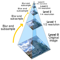
Before being put into the Convolutional Neural Network (CNN) multiple scaled versions of the image are generated. The set of these scaled images is called a pyramid. There were three different scale outputs of the image created, in a similar manner shown in the picture below
The scaling can be done by different transforms; the paper suggests to use the Laplacian transform. The Laplacian is the sum of partial second derivatives [math]\displaystyle{ \nabla^2 f = \frac{\partial^2 f}{\partial x^2} + \frac{\partial^2 f}{\partial y^2} }[/math]. A two-dimensional discrete approximation is given by the matrix [math]\displaystyle{ \left[\begin{array}{ccc}0 & 1 & 0 \\ 1 & -4 & 1 \\ 0 & 1 & 0\end{array}\right] }[/math].
Network Architecture
A typical three layer (convolution of kernel with feature map, non-linearity, pooling) CNN architecture was used. The function tanh served as the non-linearity. The kernel being used were 7x7 Toeplitz matrices (matrices with constant values along their diagonals). The pooling operation was performed by the 2x2 max-pool operator.
The same network was applied to all three different sized images. Since the parameters were shared between the networks, the same connection weights were applied to all of the images, thus allowing for the detection of scale-invariant features.
Stochastic gradient descent was used for training the filters. To avoid over-fitting the training images were edited via jitter, horizontal flipping, rotations between +8 and -8, and rescaling between 90 and 110%. The objective function was the cross entropy loss function, [which is a way to take into account the closeness of a prediction into the error https://jamesmccaffrey.wordpress.com/2013/11/05/why-you-should-use-cross-entropy-error-instead-of-classification-error-or-mean-squared-error-for-neural-network-classifier-training/].
Post-Processing
Unlike previous approaches, the emphasis of this scene-labelling method was to rely on a highly accurate pixel labelling system. So, despite the fact that a variety of approaches were attempted, including SuperPixels, Conditional Random Fields and gPb, the simple approach of super-pixels yielded state of the art results.
SuperPixels are randomly generated chunks of pixels. To label these pixels, a two layer neural network was used. Given an input of the feature vector from the CNN, the features were then averaged across the super-pixels. The picture below shows the general approach>
Results
The network was tested on the Stanford Background, SIFT Flow and Barcelona datasets.
The Stanford Background dataset shows that super-pixels could achieve state of the art results with minimal processing times.
Since super-pixels were shown to be so effective in the Stanford Dataset, they were the only method of image segmentation used for the SIFT Flow and Barcelona datasets. Instead, exposure of features to the network (whether balanced as super-index 1 or natural as super-index 2) were explored, in conjunction with the [Graph Based Segmentation http://fcv2011.ulsan.ac.kr/files/announcement/413/IJCV(2004)%20Efficient%20Graph-Based%20Image%20Segmentation.pdf] method.
From the sift dataset, it can be seen that the Graph Based Segmentation method offers a significant advantage.
In the Barcelona dataset, it can be seen that a dataset with many labels is too difficult for the CNN.
Conclusions
A wide window for contextual information, achieved through the multiscale network, improves the results largely and diminishes the role of the post-processing stage. This allows to replace the computational expensive post-processing with a simpler and faster method (e.g., majority vote) to increase the efficiency without a relevant loss in classification accuracy.
Future Work
Aside from the usual advances to CNN architecture, such as unsupervised pre-training, rectifying non-linearities and local contrast normalization, there would be a significant benefit, especially in datasets with many variables, to have a semantic understanding of the variables. For example, understanding that a window if often part of a building or a car.
