stat341 / CM 361

Computational Statistics and Data Analysis is a course offered at the University of Waterloo
Spring 2009
Instructor: Ali Ghodsi

Sampling (Generating random numbers)

Lecture of May 12th, 2009

Generating random numbers in a computational setting presents challenges. A good way to generate random numbers in computational statistics involves analyzing various distributions using computational methods. As a result, the probability distribution of each possible number appears to be uniform (pseudo-random). Outside a computational setting, presenting a uniform distribution is fairly easy (for example, rolling a fair die repetitively to produce a series of random numbers from 1 to 6).

We begin by considering the simplest case: the uniform distribution.

Multiplicative Congruential Method

One way to generate pseudo random numbers from the uniform distribution is using the Multiplicative Congruential Method. This involves three integer parameters a, b, and m, and a seed variable x₀. This method deterministically generates a sequence of numbers (based on the seed) with a seemingly random distribution (with some caveats). It proceeds as follows:

[math]\displaystyle{ x_{i+1} = (ax_{i} + b) \mod{m} }[/math]

For example, with a = 13, b = 0, m = 31, x₀ = 1, we have:

[math]\displaystyle{ x_{i+1} = 13x_{i} \mod{31} }[/math]

So,

[math]\displaystyle{ \begin{align} x_{0} &{}= 1 \end{align} }[/math]

[math]\displaystyle{ \begin{align} x_{1} &{}= 13 \times 1 + 0 \mod{31} = 13 \\ \end{align} }[/math]

[math]\displaystyle{ \begin{align} x_{2} &{}= 13 \times 13 + 0 \mod{31} = 14 \\ \end{align} }[/math]

[math]\displaystyle{ \begin{align} x_{3} &{}= 13 \times 14 + 0 \mod{31} =27 \\ \end{align} }[/math]

etc.

The above generator of pseudorandom numbers is called a Mixed Congruential Generator or Linear Congruential Generator, as they involve both an additive and a muliplicative term. For correctly chosen values of a, b, and m, this method will generate a sequence of integers including all integers between 0 and m - 1. Scaling the output by dividing the terms of the resulting sequence by m - 1, we create a sequence of numbers between 0 and 1, which is similar to sampling from a uniform distribution.

Of course, not all values of a, b, and m will behave in this way, and will not be suitable for use in generating pseudo random numbers.

For example, with a = 3, b = 2, m = 4, x₀ = 1, we have:

[math]\displaystyle{ x_{i+1} = (3x_{i} + 2) \mod{4} }[/math]

So,

[math]\displaystyle{ \begin{align} x_{0} &{}= 1 \end{align} }[/math]

[math]\displaystyle{ \begin{align} x_{1} &{}= 3 \times 1 + 2 \mod{4} = 1 \\ \end{align} }[/math]

[math]\displaystyle{ \begin{align} x_{2} &{}= 3 \times 1 + 2 \mod{4} = 1 \\ \end{align} }[/math]

etc.

For an ideal situation, we want m to be a very large prime number, [math]\displaystyle{ x_{n}\not= 0 }[/math] for any n, and the period is equal to m-1. In practice, it has been found by a paper published in 1988 by Park and Miller, that a = 7⁵, b = 0, and m = 2³¹ - 1 = 2147483647 (the maximum size of a signed integer in a 32-bit system) are good values for the Multiplicative Congruential Method.

Java's Random class is based on a generator with a = 25214903917, b = 11, and m = 2⁴⁸<ref>http://java.sun.com/javase/6/docs/api/java/util/Random.html#next(int)</ref>. The class returns at most 32 leading bits from each x_i, so it is possible to get the same value twice in a row, (when x₀ = 18698324575379, for instance) without repeating it forever.

General Methods

Since the Multiplicative Congruential Method can only be used for the uniform distribution, other methods must be developed in order to generate pseudo random numbers from other distributions.

Inverse Transform Method

This method uses the fact that when a random sample from the uniform distribution is applied to the inverse of a cumulative density function (cdf) of some distribution, the result is a random sample of that distribution. This is shown by this theorem:

Theorem:

If [math]\displaystyle{ U \sim~ \mathrm{Unif}[0, 1] }[/math] is a random variable and [math]\displaystyle{ X = F^{-1}(U) }[/math], where F is continuous, monotonic, and is the cumulative density function (cdf) for some distribution, then the distribution of the random variable X is given by F(X).

Proof:

Recall that, if f is the pdf corresponding to F, then,

[math]\displaystyle{ F(x) = P(X \leq x) = \int_{-\infty}^x f(x) }[/math]

So F is monotonically increasing, since the probability that X is less than a greater number must be greater than the probability that X is less than a lesser number.

Note also that in the uniform distribution on [0, 1], we have for all a within [0, 1], [math]\displaystyle{ P(U \leq a) = a }[/math].

So,

[math]\displaystyle{ \begin{align} P(F^{-1}(U) \leq x) &{}= P(F(F^{-1}(U)) \leq F(x)) \\ &{}= P(U \leq F(x)) \\ &{}= F(x) \end{align} }[/math]

Completing the proof.

Procedure (Continuous Case)

This method then gives us the following procedure for finding pseudo random numbers from a continuous distribution:

• Step 1: Draw [math]\displaystyle{ U \sim~ Unif [0, 1] }[/math].
• Step 2: Compute [math]\displaystyle{ X = F^{-1}(U) }[/math].

Example:

Suppose we want to draw a sample from [math]\displaystyle{ f(x) = \lambda e^{-\lambda x} }[/math] where [math]\displaystyle{ x \gt 0 }[/math] (the exponential distribution).

We need to first find [math]\displaystyle{ F(x) }[/math] and then its inverse, [math]\displaystyle{ F^{-1} }[/math].

[math]\displaystyle{ F(x) = \int^x_0 \theta e^{-\theta u} du = 1 - e^{-\theta x} }[/math]

[math]\displaystyle{ F^{-1}(x) = \frac{-\log(1-y)}{\theta} = \frac{-\log(u)}{\theta} }[/math]

Now we can generate our random sample [math]\displaystyle{ i=1\dots n }[/math] from [math]\displaystyle{ f(x) }[/math] by:

[math]\displaystyle{ 1)\ u_i \sim Unif[0, 1] }[/math]

[math]\displaystyle{ 2)\ x_i = \frac{-\log(u_i)}{\theta} }[/math]

The [math]\displaystyle{ x_i }[/math] are now a random sample from [math]\displaystyle{ f(x) }[/math].

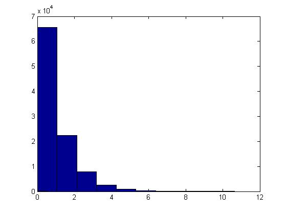
This example can be illustrated in Matlab using the code below. Generate [math]\displaystyle{ u_i }[/math], calculate [math]\displaystyle{ x_i }[/math] using the above formula and letting [math]\displaystyle{ \theta=1 }[/math], plot the histogram of [math]\displaystyle{ x_i }[/math]'s for [math]\displaystyle{ i=1,...,100,000 }[/math].

u=rand(1,100000);
x=-log(1-u)/1;
hist(x)

The histogram shows exponential pattern as expected.

The major problem with this approach is that we have to find [math]\displaystyle{ F^{-1} }[/math] and for many distributions it is too difficult (or impossible) to find the inverse of [math]\displaystyle{ F(x) }[/math]. Further, for some distributions it is not even possible to find [math]\displaystyle{ F(x) }[/math] (i.e. a closed form expression for the distribution function, or otherwise; even if the closed form expression exists, it's usually difficult to find [math]\displaystyle{ F^{-1} }[/math]).

Procedure (Discrete Case)

The above method can be easily adapted to work on discrete distributions as well.

In general in the discrete case, we have [math]\displaystyle{ x_0, \dots , x_n }[/math] where:

[math]\displaystyle{ \begin{align}P(X = x_i) &{}= p_i \end{align} }[/math]

[math]\displaystyle{ x_0 \leq x_1 \leq x_2 \dots \leq x_n }[/math]

[math]\displaystyle{ \sum p_i = 1 }[/math]

Thus we can define the following method to find pseudo random numbers in the discrete case (note that the less-than signs from class have been changed to less-than-or-equal-to signs by me, since otherwise the case of [math]\displaystyle{ U = 1 }[/math] is missed):

• Step 1: Draw [math]\displaystyle{ U~ \sim~ Unif [0,1] }[/math].
• Step 2:
  • If [math]\displaystyle{ U \lt p_0 }[/math], return [math]\displaystyle{ X = x_0 }[/math]
  • If [math]\displaystyle{ p_0 \leq U \lt p_0 + p_1 }[/math], return [math]\displaystyle{ X = x_1 }[/math]
  • ...
  • In general, if [math]\displaystyle{ p_0+ p_1 + \dots + p_{k-1} \leq U \lt p_0 + \dots + p_k }[/math], return [math]\displaystyle{ X = x_k }[/math]

Example (from class):

Suppose we have the following discrete distribution:

[math]\displaystyle{ \begin{align} P(X = 0) &{}= 0.3 \\ P(X = 1) &{}= 0.2 \\ P(X = 2) &{}= 0.5 \end{align} }[/math]

The cumulative density function (cdf) for this distribution is then:

[math]\displaystyle{ F(x) = \begin{cases} 0, & \text{if } x \lt 0 \\ 0.3, & \text{if } 0 \leq x \lt 1 \\ 0.5, & \text{if } 1 \leq x \lt 2 \\ 1, & \text{if } 2 \leq x \end{cases} }[/math]

Then we can generate numbers from this distribution like this, given [math]\displaystyle{ u_0, \dots, u_n }[/math] from [math]\displaystyle{ U \sim~ Unif[0, 1] }[/math]:

[math]\displaystyle{ x_i = \begin{cases} 0, & \text{if } u_i \leq 0.3 \\ 1, & \text{if } 0.3 \lt u_i \leq 0.5 \\ 2, & \text{if } 0.5 \lt u_i \leq 1 \end{cases} }[/math]

This example can be illustrated in Matlab using the code below:

p=[0.3,0.2,0.5];
for i=1:1000;
  u=rand;
  if u <= p(1)
    x(i)=0;
  elseif u < sum(p(1,2))
    x(i)=1;
  else
    x(i)=2;
  end
end

Lecture of May 14th, 2009

Today, we continue the discussion on sampling (generating random numbers) from general distributions with the Acceptance/Rejection Method.

Acceptance/Rejection Method

Suppose we wish to sample from a target distribution [math]\displaystyle{ f(x) }[/math] that is difficult or impossible to sample from directly. Suppose also that we have a proposal distribution [math]\displaystyle{ g(x) }[/math] from which we have a reasonable method of sampling (e.g. the uniform distribution). Then, if there is a constant [math]\displaystyle{ c \ |\ c \cdot g(x) \geq f(x)\ \forall x }[/math], accepting samples drawn in successions from [math]\displaystyle{ c \cdot g(x) }[/math] with ratio [math]\displaystyle{ \frac {f(x)}{c \cdot g(x)} }[/math] close to 1 will yield a sample that follows the target distribution [math]\displaystyle{ f(x) }[/math]; on the other hand we would reject the samples if the ratio is not close to 1.

The following graph shows the pdf of [math]\displaystyle{ f(x) }[/math] and [math]\displaystyle{ c \cdot g(x) }[/math]

File:fxcgx.JPG

At x=7; sampling from [math]\displaystyle{ c \cdot g(x) }[/math] will yield a sample that follows the target distribution [math]\displaystyle{ f(x) }[/math]

At x=9; we will reject samples according to the ratio [math]\displaystyle{ \frac {f(x)}{c \cdot g(x)} }[/math] after sampling from [math]\displaystyle{ c \cdot g(x) }[/math]

Proof

Note the following:

• [math]\displaystyle{ Pr(X|accept) = \frac{Pr(accept|X) \times Pr(X)}{Pr(accept)} }[/math] (Bayes' theorem)
• [math]\displaystyle{ Pr(accept|X) = \frac{f(x)}{c \cdot g(x)} }[/math]
• [math]\displaystyle{ Pr(X) = g(x)\frac{}{} }[/math]

So, [math]\displaystyle{ Pr(accept) = \int^{}_x Pr(accept|X) \times Pr(X) dx }[/math] [math]\displaystyle{ = \int^{}_x \frac{f(x)}{c \cdot g(x)} g(x) dx }[/math] [math]\displaystyle{ = \frac{1}{c} \int^{}_x f(x) dx }[/math] [math]\displaystyle{ = \frac{1}{c} }[/math]

Therefore, [math]\displaystyle{ Pr(X|accept) = \frac{\frac{f(x)}{c\ \cdot g(x)} \times g(x)}{\frac{1}{c}} = f(x) }[/math] as required.

Procedure (Continuous Case)

• Choose [math]\displaystyle{ g(x) }[/math] (a density function that is simple to sample from)
• Find a constant c such that :[math]\displaystyle{ c \cdot g(x) \geq f(x) }[/math]

1. Let [math]\displaystyle{ Y \sim~ g(y) }[/math]
2. Let [math]\displaystyle{ U \sim~ Unif [0,1] }[/math]
3. If [math]\displaystyle{ U \leq \frac{f(x)}{c \cdot g(x)} }[/math] then X=Y; else reject and go to 1

Example:

Suppose we want to sample from Beta(2,1), for [math]\displaystyle{ 0 \leq x \leq 1 }[/math]. Recall:

[math]\displaystyle{ Beta(2,1) = \frac{\Gamma (2+1)}{\Gamma (2) \Gamma(1)} \times x^1(1-x)^0 = \frac{2!}{1!0!} \times x = 2x }[/math]

• Choose [math]\displaystyle{ g(x) \sim~ Unif [0,1] }[/math]
• Find c: c = 2 (see notes below)

1. Let [math]\displaystyle{ Y \sim~ Unif [0,1] }[/math]
2. Let [math]\displaystyle{ U \sim~ Unif [0,1] }[/math]
3. If [math]\displaystyle{ U \leq \frac{2Y}{2} = Y }[/math], then X=Y; else go to 1

[math]\displaystyle{ c }[/math] was chosen to be 2 in this example since [math]\displaystyle{ \max \left(\frac{f(x)}{g(x)}\right) }[/math] in this example is 2. This condition is important since it helps us in finding a suitable [math]\displaystyle{ c }[/math] to apply the Acceptance/Rejection Method.

In MATLAB, the code that demonstrates the result of this example is:

   j = 1;
       while i < 1000
           y = rand;
           u = rand;
           if u <= y
               x(j) = y;
               j = j + 1;
               i = i + 1;
           end
       end
       hist(x);
       

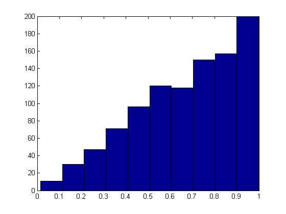
The histogram produced here should follow the target distribution, [math]\displaystyle{ f(x) = 2x }[/math], for the interval [math]\displaystyle{ 0 \leq x \leq 1 }[/math].

The histogram shows the PDF of a Beta(2,1) distribution as expected.

The Discrete Case

The Acceptance/Rejection Method can be extended for discrete target distributions. The difference compared to the continuous case is that the proposal distribution [math]\displaystyle{ g(x) }[/math] must also be discrete distribution. For our purposes, we can consider g(x) to be a discrete uniform distribution on the set of values that X may take on in the target distribution.

Example

Suppose we want to sample from a distribution with the following probability mass function (pmf):

P(X=1) = 0.15
P(X=2) = 0.55
P(X=3) = 0.20
P(X=4) = 0.10 

• Choose [math]\displaystyle{ g(x) }[/math] to be the discrete uniform distribution on the set [math]\displaystyle{ \{1,2,3,4\} }[/math]
• Find c: [math]\displaystyle{ c = \max \left(\frac{f(x)}{g(x)} \right)= 0.55/0.25 = 2.2 }[/math]

1. Generate [math]\displaystyle{ Y \sim~ Unif \{1,2,3,4\} }[/math]
2. Let [math]\displaystyle{ U \sim~ Unif [0,1] }[/math]
3. If [math]\displaystyle{ U \leq \frac{f(x)}{2.2 \times 0.25} }[/math], then X=Y; else go to 1

Limitations

If the proposed distribution is very different from the target distribution, we may have to rejected a large number of points before a good sample size of the target distribution can be established. It may also be difficult to find such [math]\displaystyle{ g(x) }[/math] that satisfies all the conditions of the procedure.

We will now begin to discuss sampling from specific distributions.

Special Technique for sampling from Gamma Distribution

Recall that the cdf of the Gamma distribution is:

[math]\displaystyle{ F(x) = \int_0^{\lambda x} \frac{e^{-y}y^{t-1}}{(t-1)!} dy }[/math]

If we wish to sample from this distribution, it will be difficult for both the Inverse Method and the Acceptance/Rejection Method.

Additive Property of Gamma Distribution

Recall that if [math]\displaystyle{ X_1, \dots, X_t }[/math] are independent exponential distributions with mean [math]\displaystyle{ \lambda }[/math] (in other words, [math]\displaystyle{ X_i\sim~ Exp (\lambda) }[/math]), then [math]\displaystyle{ \Sigma_{i=1}^t X_i \sim~ Gamma (t, \lambda) }[/math]

It appears that if we want to sample from the Gamma distribution, we can consider sampling from t independent exponential distributions with mean [math]\displaystyle{ \lambda }[/math] (using the Inverse Method) and add them up. Details will be discussed in the next lecture.

Lecture of May 19th, 2009

We have examined two general techniques for sampling from distributions. However, for certain distributions more practical methods exist. We will now look at two cases,
Gamma distributions and Normal distributions, where such practical methods exist.

Gamma Distribution

Given the additive property of the gamma distribution,

If [math]\displaystyle{ X_1, \dots, X_t }[/math] are independent random variables with [math]\displaystyle{ X_i\sim~ Exp (\lambda) }[/math] then,

[math]\displaystyle{ \Sigma_{i=1}^t X_i \sim~ Gamma (t, \lambda) }[/math]

we can use the following procedure using the inverse method and independent uniform samples seen before to generate a sample following a Gamma distribution.

Procedure

1. Sample independently from a uniform distribution [math]\displaystyle{ t }[/math] times, giving [math]\displaystyle{ u_1,\dots,u_t }[/math]
2. Sample independently from an exponential distribution [math]\displaystyle{ t }[/math] times, giving [math]\displaystyle{ x_1,\dots,x_t }[/math] such that,
   [math]\displaystyle{ \begin{align} x_1 \sim~ Exp(\lambda)\\ \vdots \\ x_t \sim~ Exp(\lambda) \end{align} }[/math]
   
   This can be given by the inverse method,
   [math]\displaystyle{ \begin{align} x_i = -\frac {1}{\lambda}\log(u_i) \end{align} }[/math]
3. Using the additive property,
   [math]\displaystyle{ \begin{align} X &{}= -\frac {1}{\lambda}\log(u_1) - \frac {1}{\lambda}\log(u_2) \dots - \frac {1}{\lambda}\log(u_t) \\ X &{}= -\frac {1}{\lambda}\log(\prod_{i=1}^{t}u_i) \sim~ Gamma (t, \lambda) \end{align} }[/math]

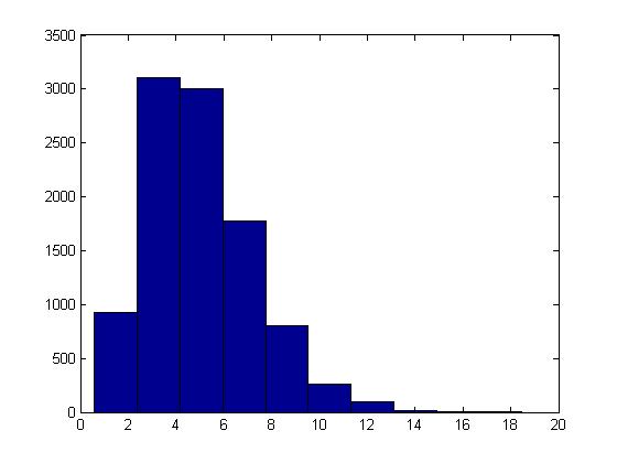
This proceedure can be illustrated in Matlab using the code below with [math]\displaystyle{ t = 5, \lambda = 1 }[/math] :

U = rand(10000,5);
X = sum( -log(U), 2);
hist(X)

Normal Distribution

The cdf for the Standard Normal distribution is:

[math]\displaystyle{ F(Z) = \int_{-\infty}^{Z}\frac{1}{2\pi}e^{-x^2/2}dx }[/math]

We can see that the normal distribution is difficult to sample from using the general methods so far, eg. the inverse is not easy to obtain from F(Z). However, specific methods exist for sampling from the Standard Normal distribution.

Box-Muller Method

The Box-Muller or Polar method uses an approach where we have one space that is easy to sample in, and another with the desired distribution under a transformation. If we know such a transformation for the Standard Normal, then all we have to do is transform our easy sample to obtain a sample from the Standard Normal distribution.

Properties of Polar and Cartesian Coordinates

If x,y are points on the cartesian plane, r the length of the radius from a point in the polar plane to the pole, and θ the angle formed with the polar axis then,

• [math]\displaystyle{ \begin{align} r^2 = x^2 + y^2 \end{align} }[/math]
• [math]\displaystyle{ \tan(\theta) = \frac{y}{x} }[/math]

• [math]\displaystyle{ \begin{align} x = \cos(\theta) \end{align} }[/math]
• [math]\displaystyle{ \begin{align} y = \sin(\theta) \end{align} }[/math]

Let x and y be independent with a standard normal distribution,

[math]\displaystyle{ x \sim~ N(0,1) }[/math]

[math]\displaystyle{ y \sim~ N(0,1) }[/math]

also, let r and θ be the polar coordinates of (x,y). Then the joint distribution of independent x and y is given by,

[math]\displaystyle{ \begin{align} f(x,y) = f(x)f(y) &{}= \frac{1}{\sqrt{2\pi}}e^{-\frac{x^2}{2}}\frac{1}{\sqrt{2\pi}}e^{-\frac{y^2}{2}} \\ &{}=\frac{1}{2\pi}e^{-\frac{x^2+y^2}{2}} \end{align} }[/math]

It can also be shown that the joint distribution of r and θ is given by,

[math]\displaystyle{ \begin{matrix} f(r,\theta) = \frac{1}{2}e^{-\frac{d}{2}}*\frac{1}{2\pi},\quad d = r^2 \end{matrix} }[/math]

[math]\displaystyle{ \begin{matrix} \Rightarrow \frac{1}{2}e^{-\frac{d}{2}} \sim~ exp(1/2), \quad \frac{1}{2\pi} \sim~ Unif[0,2\pi] \end{matrix} }[/math]