stat841f10: Difference between revisions
No edit summary |
|||
| Line 808: | Line 808: | ||
==Fisher's Linear Discriminant Analysis (FDA) October 5, 2010== | ==Fisher's Linear Discriminant Analysis (FDA) October 5, 2010== | ||
===Lecture Summary === | |||
In This lecture introduces Fisher's Discriminant Analysis method. While discussing the goals specified by Fisher for his analysis. Then proceeding by mathematical formulation of these goals. The lecture summarizes the topic with General solution that satisfies these goals. | |||
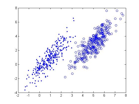
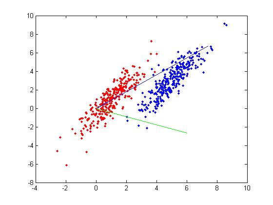
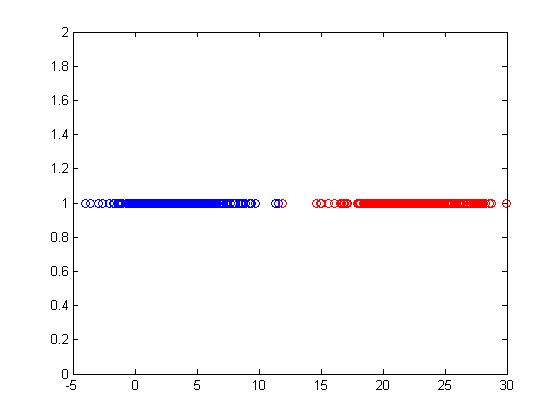
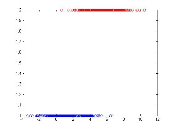
[[File:graph.jpg|500px|thumb|right| PCA vs FDA]] | |||
Fisher's Discriminant Analysis (FDA), also known as Fisher's Linear Discriminant Analysis (LDA) in some sources, is a classical feature extraction technique. It was originally described in 1936 by Sir [http://en.wikipedia.org/wiki/Ronald_A._Fisher Ronald Aylmer Fisher], an English statistician and eugenicist who has been described as one of the founders of modern statistical science. His original paper describing FDA can be found [http://digital.library.adelaide.edu.au/dspace/handle/2440/15227 here]; a Wikipedia article summarizing the algorithm can be found [http://en.wikipedia.org/wiki/Linear_discriminant_analysis#Fisher.27s_linear_discriminant here]. | Fisher's Discriminant Analysis (FDA), also known as Fisher's Linear Discriminant Analysis (LDA) in some sources, is a classical feature extraction technique. It was originally described in 1936 by Sir [http://en.wikipedia.org/wiki/Ronald_A._Fisher Ronald Aylmer Fisher], an English statistician and eugenicist who has been described as one of the founders of modern statistical science. His original paper describing FDA can be found [http://digital.library.adelaide.edu.au/dspace/handle/2440/15227 here]; a Wikipedia article summarizing the algorithm can be found [http://en.wikipedia.org/wiki/Linear_discriminant_analysis#Fisher.27s_linear_discriminant here]. | ||
Revision as of 14:53, 5 October 2010
Editor sign up
Classfication-2010.09.21
Lecture Summary
- Classification is an area of supervised learning that systematically assigns an unlabeled novel data to their label through the characteristics and attributes obtained from observation.
- Classification is the prediction of a discrete random variable [math]\displaystyle{ \mathcal{Y} }[/math] from another random variable [math]\displaystyle{ \mathcal{X} }[/math], where [math]\displaystyle{ \mathcal{Y} }[/math] represents the label assigned to a new data input and [math]\displaystyle{ \mathcal{X} }[/math] represents the known feature values of the input. The classification rule used by a classifier has the form [math]\displaystyle{ \,h: \mathcal{X} \mapsto \mathcal{Y} }[/math].
- True error rate is the probability that the classification rule [math]\displaystyle{ \,h }[/math] does not correctly classify any data input. Empirical error rate is the frequency where the classification rule [math]\displaystyle{ \,h }[/math] does not correctly classify any data input in the training set. In experimental tasks true error cannot be measured and as a result the empirical error rate is used as the estimate.
- Bayes Classifier is a probabilistic classifier by applying Bayes Theorem with strong (naive) independence assumptions. It has the advantage of requiring small training data to estimate the parameters needed for classification. Under this classifier an input [math]\displaystyle{ \,x }[/math] is classified to class [math]\displaystyle{ \,y }[/math] where the posterior probability for [math]\displaystyle{ \,y }[/math] is the largest for input [math]\displaystyle{ \,x }[/math].
- Bayes Classification Rule Optimality Theorem states that Bayes classifier is the optimal classifier, in other words the true error rate of the Bayes classification rule will always be smaller or equal to any other classification rule
- Bayes Decision Boundary is the hyperplane boundary that separates the two classes [math]\displaystyle{ \,m, n }[/math] obtained by setting the posterior probability for the two classes equal, [math]\displaystyle{ \,D(h)=\{x: P(Y=m|X=x)=P(Y=n|X=x)\} }[/math].
- Linear Discriminant Analysis (LDA) for the Bayes classifier decision boundary between two classes makes the assumption that both are generated from Gaussian distribution and have the same covariance matrix.
Classification
{{
Template:namespace detect
| type = style | image = | imageright = | style = | textstyle = | text = This article may require cleanup to meet Wikicoursenote's quality standards. The specific problem is: Each topic should begin with a short summary as a separated section. Please write a digest for each topic. Please improve this article if you can. (29 September 2010) | small = | smallimage = | smallimageright = | smalltext = }}
Statistical classification, or simply known as classification, is an area of supervised learning that addresses the problem of how to systematically assign unlabeled (classes unknown) novel data to their labels (classes or groups or types) by using knowledge of their features (characteristics or attributes) that are obtained from observation and/or measurement. A classifier is a specific technique or method for performing classification. To classify new data, a classifier first uses labeled (classes are known) training data to train a model, and then it uses a function known as its classification rule to assign a label to each new data input after feeding the input's known feature values into the model to determine how much the input belongs to each class.
Classification has been an important task for people and society since the beginnings of history. According to this link, the earliest application of classification in human society was probably done by prehistory peoples for recognizing which wild animals were beneficial to people and which one were harmful, and the earliest systematic use of classification was done by the famous Greek philosopher Aristotle (384BC - 322 BC) when he, for example, grouped all living things into the two groups of plants and animals. Classification is generally regarded as one of four major areas of statistics, with the other three major areas being regression regression, clustering, and dimensionality reduction (feature extraction or manifold learning). Please be noted that some people consider classification to be a broad area that consists supervised and unsupervised methods of classifying data. In this view, as can be seen in this link, clustering is simply a special case of classification and it may be called unsupervised classification.
In classical statistics, classification techniques were developed to learn useful information using small data sets where there is usually not enough of data. When machine learning was developed after the application of computers to statistics, classification techniques were developed to work with very large data sets where there is usually too many data. A major challenge facing data mining using machine learning is how to efficiently find useful patterns in very large amounts of data. An interesting quote that describes this problem quite well is the following one made by the retired Yale University Librarian Rutherford D. Rogers.
       "We are drowning in information and starving for knowledge."
                                                         - Rutherford D. Rogers
In the Information Age, machine learning when it is combined with efficient classification techniques can be very useful for data mining using very large data sets. This is most useful when the structure of the data is not well understood but the data nevertheless exhibit strong statistical regularity. Areas in which machine learning and classification have been successfully used together include search and recommendation (e.g. Google, Amazon), automatic speech recognition and speaker verification, medical diagnosis, analysis of gene expression, drug discovery etc.
The formal mathematical definition of classification is as follows:
Definition: Classification is the prediction of a discrete random variable [math]\displaystyle{ \mathcal{Y} }[/math] from another random variable [math]\displaystyle{ \mathcal{X} }[/math], where [math]\displaystyle{ \mathcal{Y} }[/math] represents the label assigned to a new data input and [math]\displaystyle{ \mathcal{X} }[/math] represents the known feature values of the input.
A set of training data used by a classifier to train its model consists of [math]\displaystyle{ \,n }[/math] independently and identically distributed (i.i.d) ordered pairs [math]\displaystyle{ \,\{(X_{1},Y_{1}), (X_{2},Y_{2}), \dots , (X_{n},Y_{n})\} }[/math], where the values of the [math]\displaystyle{ \,ith }[/math] training input's feature values [math]\displaystyle{ \,X_{i} = (\,X_{i1}, \dots , X_{id}) \in \mathcal{X} \subset \mathbb{R}^{d} }[/math] is a d-dimensional vector and the label of the [math]\displaystyle{ \, ith }[/math] training input is [math]\displaystyle{ \,Y_{i} \in \mathcal{Y} }[/math] that takes a finite number of values. The classification rule used by a classifier has the form [math]\displaystyle{ \,h: \mathcal{X} \mapsto \mathcal{Y} }[/math]. After the model is trained, each new data input whose feature values is [math]\displaystyle{ \,x }[/math] is given the label [math]\displaystyle{ \,\hat{Y}=h(x) }[/math].
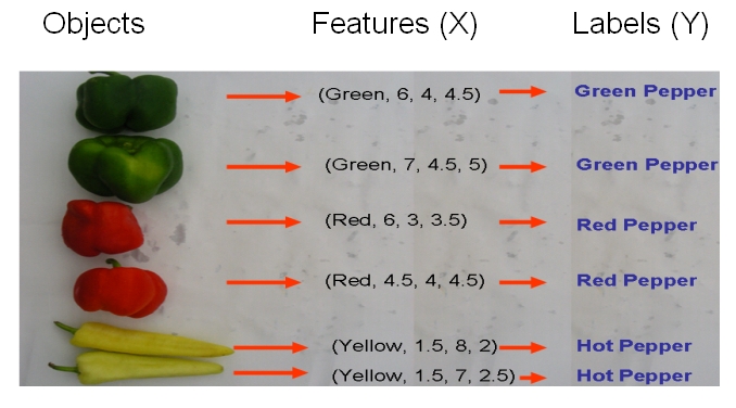
As an example, if we would like to classify some vegetables and fruits, then our training data might look something like the one shown in the following picture from Professor Ali Ghodsi's Fall 2010 STAT 841 slides.
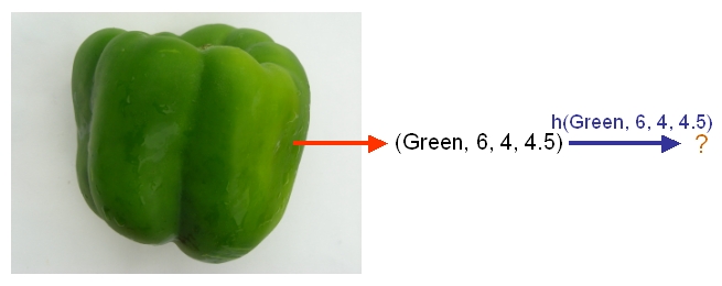
After we have selected a classifier and then built our model using our training data, we could use the classifier's classification rule [math]\displaystyle{ \ h }[/math] to classify any newly-given vegetable or fruit such as the one shown in the following picture from Professor Ali Ghodsi's Fall 2010 STAT 841 slides after first obtaining its feature values.
As another example, suppose we wish to classify newly-given fruits into apples and oranges by considering three features of a fruit that comprise its color, its diameter, and its weight. After selecting a classifier and constructing a model using training data [math]\displaystyle{ \,\{(X_{color, 1}, X_{diameter, 1}, X_{weight, 1}, Y_{1}), \dots , (X_{color, n}, X_{diameter, n}, X_{weight, n}, Y_{n})\} }[/math], we could then use the classifier's classification rule [math]\displaystyle{ \,h }[/math] to assign any newly-given fruit having known feature values [math]\displaystyle{ \,x = (\,x_{color}, x_{diameter} , x_{weight}) }[/math] the label [math]\displaystyle{ \, \hat{Y}=h(x) \in \mathcal{Y}= \{apple,orange\} }[/math].
Error rate
{{
Template:namespace detect
| type = style | image = | imageright = | style = | textstyle = | text = This article may require cleanup to meet Wikicoursenote's quality standards. The specific problem is: It is important to notice why do we use empirical error rate instead of true error rate and why do we define it. The main reason is that in experimental tasks we can't measure true error rate and we estimate it by empirical error rate which is unbiased estimation of true error rate. Please improve this article if you can. (October 2nd 2010) | small = | smallimage = | smallimageright = | smalltext = }} The true error rate' [math]\displaystyle{ \,L(h) }[/math] of a classifier having classification rule [math]\displaystyle{ \,h }[/math] is defined as the probability that [math]\displaystyle{ \,h }[/math] does not correctly classify any new data input, i.e., it is defined as [math]\displaystyle{ \,L(h)=P(h(X) \neq Y) }[/math]. Here, [math]\displaystyle{ \,X \in \mathcal{X} }[/math] and [math]\displaystyle{ \,Y \in \mathcal{Y} }[/math] are the known feature values and the true class of that input, respectively.
The empirical error rate (or training error rate) of a classifier having classification rule [math]\displaystyle{ \,h }[/math] is defined as the frequency at which [math]\displaystyle{ \,h }[/math] does not correctly classify the data inputs in the training set, i.e., it is defined as [math]\displaystyle{ \,\hat{L}_{n} = \frac{1}{n} \sum_{i=1}^{n} I(h(X_{i}) \neq Y_{i}) }[/math], where [math]\displaystyle{ \,I }[/math] is an indicator variable and [math]\displaystyle{ \,I = \left\{\begin{matrix} 1 &\text{if } h(X_i) \neq Y_i \\ 0 &\text{if } h(X_i) = Y_i \end{matrix}\right. }[/math]. Here, [math]\displaystyle{ \,X_{i} \in \mathcal{X} }[/math] and [math]\displaystyle{ \,Y_{i} \in \mathcal{Y} }[/math] are the known feature values and the true class of the [math]\displaystyle{ \,ith }[/math] training input, respectively.
Bayes Classifier
A Bayes classifier is a simple probabilistic classifier based on applying Bayes' theorem (from Bayesian statistics) with strong (naive) independence assumptions. A more descriptive term for the underlying probability model would be "independent feature model".
In simple terms, a Bayes classifier assumes that the presence (or absence) of a particular feature of a class is unrelated to the presence (or absence) of any other feature. For example, a fruit may be considered to be an apple if it is red, round, and about 4" in diameter. Even if these features depend on each other or upon the existence of the other features, a Bayes classifier considers all of these properties to independently contribute to the probability that this fruit is an apple.
Depending on the precise nature of the probability model, naive Bayes classifiers can be trained very efficiently in a supervised learning setting. In many practical applications, parameter estimation for Bayes models uses the method of maximum likelihood; in other words, one can work with the naive Bayes model without believing in Bayesian probability or using any Bayesian methods.
In spite of their design and apparently over-simplified assumptions, naive Bayes classifiers have worked quite well in many complex real-world situations. In 2004, analysis of the Bayesian classification problem has shown that there are some theoretical reasons for the apparently unreasonable efficacy of Bayes classifiers.[1] Still, a comprehensive comparison with other classification methods in 2006 showed that Bayes classification is outperformed by more current approaches, such as boosted trees or random forests.[2]
An advantage of the naive Bayes classifier is that it requires a small amount of training data to estimate the parameters (means and variances of the variables) necessary for classification. Because independent variables are assumed, only the variances of the variables for each class need to be determined and not the entire covariance matrix.
After training its model using training data, the Bayes classifier classifies any new data input in two steps. First, it uses the input's known feature values and the Bayes formula to calculate the input's posterior probability of belonging to each class. Then, it uses its classification rule to place the input into its most-probable class, which is the one associated with the input's largest posterior probability.
In mathematical terms, for a new data input having feature values [math]\displaystyle{ \,(X = x)\in \mathcal{X} }[/math], the Bayes classifier labels the input as [math]\displaystyle{ (Y = y) \in \mathcal{Y} }[/math], such that the input's posterior probability [math]\displaystyle{ \,P(Y = y|X = x) }[/math] is maximum over all of the members of [math]\displaystyle{ \mathcal{Y} }[/math].
Suppose there are [math]\displaystyle{ \,k }[/math] classes and we are given a new data input having feature values [math]\displaystyle{ \,x }[/math]. The following derivation shows how the Bayes classifier finds the input's posterior probability [math]\displaystyle{ \,P(Y = y|X = x) }[/math] of belonging to each class in [math]\displaystyle{ \mathcal{Y} }[/math].
- [math]\displaystyle{ \begin{align} P(Y=y|X=x) &= \frac{P(X=x|Y=y)P(Y=y)}{P(X=x)} \\ &=\frac{P(X=x|Y=y)P(Y=y)}{\Sigma_{\forall i \in \mathcal{Y}}P(X=x|Y=i)P(Y=i)} \end{align} }[/math]
Here, [math]\displaystyle{ \,P(Y=y|X=x) }[/math] is known as the posterior probability as mentioned above, [math]\displaystyle{ \,P(Y=y) }[/math] is known as the prior probability, [math]\displaystyle{ \,P(X=x|Y=y) }[/math] is known as the likelihood, and [math]\displaystyle{ \,P(X=x) }[/math] is known as the evidence.
In the special case where there are two classes, i.e., [math]\displaystyle{ \, \mathcal{Y}=\{0, 1\} }[/math], the Bayes classifier makes use of the function [math]\displaystyle{ \,r(x)=P\{Y=1|X=x\} }[/math] which is the prior probability of a new data input having feature values [math]\displaystyle{ \,x }[/math] belonging to the class [math]\displaystyle{ \,Y = 1 }[/math]. Following the above derivation for the posterior probabilities of a new data input, the Bayes classifier calculates [math]\displaystyle{ \,r(x) }[/math] as follows:
- [math]\displaystyle{ \begin{align} r(x)&=P(Y=1|X=x) \\ &=\frac{P(X=x|Y=1)P(Y=1)}{P(X=x)}\\ &=\frac{P(X=x|Y=1)P(Y=1)}{P(X=x|Y=1)P(Y=1)+P(X=x|Y=0)P(Y=0)} \end{align} }[/math]
The Bayes classifier's classification rule [math]\displaystyle{ \,h^*: \mathcal{X} \mapsto \mathcal{Y} }[/math], then, is
- [math]\displaystyle{ \, h^*(x)= \left\{\begin{matrix} 1 &\text{if } \hat r(x)\gt \frac{1}{2} \\ 0 &\text{if } \mathrm{otherwise} \end{matrix}\right. }[/math].
Here, [math]\displaystyle{ \,x }[/math] is the feature values of a new data input and [math]\displaystyle{ \hat r(x) }[/math] is the estimated value of the function [math]\displaystyle{ \,r(x) }[/math] given by the Bayes classifier's model after feeding [math]\displaystyle{ \,x }[/math] into the model. Still in this special case of two classes, the Bayes classifier's decision boundary is defined as the set [math]\displaystyle{ \,D(h)=\{x: P(Y=1|X=x)=P(Y=0|X=x)\} }[/math]. The decision boundary [math]\displaystyle{ \,D(h) }[/math] essentially combines together the trained model and the decision function [math]\displaystyle{ \,h }[/math], and it is used by the Bayes classifier to assign any new data input to a label of either [math]\displaystyle{ \,Y = 0 }[/math] or [math]\displaystyle{ \,Y = 1 }[/math] depending on which side of the decision boundary the input lies in. From this decision boundary, it is easy to see that, in the case where there are two classes, the Bayes classifier's classification rule can be re-expressed as
- [math]\displaystyle{ \, h^*(x)= \left\{\begin{matrix} 1 &\text{if } P(Y=1|X=x)\gt P(Y=0|X=x) \\ 0 &\text{if } \mathrm{otherwise} \end{matrix}\right. }[/math].
Bayes Classification Rule Optimality Theorem
- The Bayes classifier is the optimal classifier in that it produces the least possible probability of misclassification for any given new data input, i.e., for any other classifier having classification rule [math]\displaystyle{ \,h }[/math], it is always true that [math]\displaystyle{ \,L(h^*(x)) \le L(h(x)) }[/math]. Here, [math]\displaystyle{ \,L }[/math] represents the true error rate, [math]\displaystyle{ \,h^* }[/math] is the Bayes classifier's classification rule, and [math]\displaystyle{ \,x }[/math] is any given data input's feature values.
Although the Bayes classifier is optimal in the theoretical sense, other classifiers may nevertheless outperform it in practice. The reason for this is that various components which make up the Bayes classifier's model, such as the likelihood and prior probabilities, must either be estimated using training data or be guessed with a certain degree of belief, as a result, their estimated values in the trained model may deviate quite a bit from their true population values and this ultimately can cause the posterior probabilities to deviate quite a bit from their true population values. A rather detailed proof of this theorem is available here. {{
Template:namespace detect
| type = style | image = | imageright = | style = | textstyle = | text = This article may require cleanup to meet Wikicoursenote's quality standards. The specific problem is: It must be noted if Bayes classifier is optimal why do we need to other classifiers like neural networks. The main reason is that while this method is optimal and simple it needs a lot of information if we want to implement it. We need to have the class conditional distribution, which is hard to have it and needs estimation. Basically in real applications we assume it to be a known distribution based on the problem but it is not easy in general to have the distribution of the process. We also need to know the prior and marginal probabilities, while they are more simple to get but add complexity to our problem. For this reason other classifiers have been developed. While they are not optimal but can be used more easily and need less information about the process.. Please improve this article if you can. (October 2nd 2010) | small = | smallimage = | smallimageright = | smalltext = }}
Defining the classification rule:
In the special case of two classes, the Bayes classifier can use three main approaches to define its classification rule [math]\displaystyle{ \,h }[/math]:
- 1) Empirical Risk Minimization: Choose a set of classifiers [math]\displaystyle{ \mathcal{H} }[/math] and find [math]\displaystyle{ \,h^*\in \mathcal{H} }[/math] that minimizes some estimate of the true error rate [math]\displaystyle{ \,L(h) }[/math].
- 2) Regression: Find an estimate [math]\displaystyle{ \hat r }[/math] of the function [math]\displaystyle{ x }[/math] and define
- [math]\displaystyle{ \, h(x)= \left\{\begin{matrix} 1 &\text{if } \hat r(x)\gt \frac{1}{2} \\ 0 &\text{if } \mathrm{otherwise} \end{matrix}\right. }[/math].
- 3) Density Estimation: Estimate [math]\displaystyle{ \,P(X=x|Y=0) }[/math] from the [math]\displaystyle{ \,X_{i} }[/math]'s for which [math]\displaystyle{ \,Y_{i} = 0 }[/math], estimate [math]\displaystyle{ \,P(X=x|Y=1) }[/math] from the [math]\displaystyle{ \,X_{i} }[/math]'s for which [math]\displaystyle{ \,Y_{i} = 1 }[/math], and estimate [math]\displaystyle{ \,P(Y = 1) }[/math] as [math]\displaystyle{ \,\frac{1}{n} \sum_{i=1}^{n} Y_{i} }[/math]. Then, calculate [math]\displaystyle{ \,\hat r(x) = \hat P(Y=1|X=x) }[/math] and define
- [math]\displaystyle{ \, h(x)= \left\{\begin{matrix} 1 &\text{if } \hat r(x)\gt \frac{1}{2} \\ 0 &\text{if } \mathrm{otherwise} \end{matrix}\right. }[/math].
Typically, the Bayes classifier uses approach 3 to define its classification rule. These three approaches can easily be generalized to the case where the number of classes exceeds two.
Multi-class classification:
Suppose there are [math]\displaystyle{ \,k }[/math] classes, where [math]\displaystyle{ \,k \ge 2 }[/math].
In the above discussion, we introduced the Bayes formula for this general case:
- [math]\displaystyle{ \begin{align} P(Y=y|X=x) &=\frac{P(X=x|Y=y)P(Y=y)}{\Sigma_{\forall i \in \mathcal{Y}}P(X=x|Y=i)P(Y=i)} \end{align} }[/math]
which can re-worded as:
- [math]\displaystyle{ \begin{align} P(Y=y|X=x) &=\frac{f_y(x)\pi_y}{\Sigma_{\forall i \in \mathcal{Y}} f_i(x)\pi_i} \end{align} }[/math]
Here, [math]\displaystyle{ \,f_y(x) = P(X=x|Y=y) }[/math] is known as the likelihood function and [math]\displaystyle{ \,\pi_y = P(Y=y) }[/math] is known as the prior probability.
In the general case where there are at least two classes, the Bayes classifier uses the following theorem to assign any new data input having feature values [math]\displaystyle{ \,x }[/math] into one of the [math]\displaystyle{ \,k }[/math] classes.
Theorem
- Suppose that [math]\displaystyle{ \mathcal{Y}= \{1, \dots, k\} }[/math], where [math]\displaystyle{ \,k \ge 2 }[/math]. Then, the optimal classification rule is [math]\displaystyle{ \,h^*(x) = arg max_{i} P(Y=i|X=x) }[/math], where [math]\displaystyle{ \,i \in \{1, \dots, k\} }[/math].
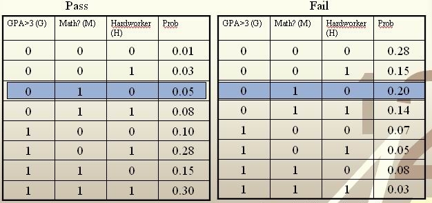
Example: We are going to predict if a particular student will pass STAT 441/841. There are two classes represented by [math]\displaystyle{ \, \mathcal{Y}\in \{ 0,1 \} }[/math], where 1 refers to pass and 0 refers to fail. Suppose that the prior probabilities are estimated or guessed to be [math]\displaystyle{ \,\hat P(Y = 1) = \hat P(Y = 0) = 0.5 }[/math]. We have data on past student performances, which we shall use to train the model. For each student, we know the following:
- Whether or not the student’s GPA was greater than 3.0 (G).
- Whether or not the student had a strong math background (M).
- Whether or not the student was a hard worker (H).
- Whether or not the student passed or failed the course.
These known data are summarized in the following tables:
{{
Template:namespace detect
| type = style | image = | imageright = | style = | textstyle = | text = This article may require cleanup to meet Wikicoursenote's quality standards. The specific problem is: These tables should be checked over to make sure that they are correct for the numerical calculation that follows. Please improve this article if you can. (September 2010) | small = | smallimage = | smallimageright = | smalltext = }}
For each student, his/her feature values is [math]\displaystyle{ \, x = \{G, M, H\} }[/math] and his or her class is [math]\displaystyle{ \, y \in \{0, 1\} }[/math].
Suppose there is a new student having feature values [math]\displaystyle{ \, x = \{0, 1, 0\} }[/math], and we would like to predict whether he/she would pass the course. [math]\displaystyle{ \,\hat r(x) }[/math] is found as follows:
{{
Template:namespace detect
| type = style | image = | imageright = | style = | textstyle = | text = This article may require cleanup to meet Wikicoursenote's quality standards. The specific problem is: The following calculation needs to be checked over since I am not sure if it is entirely correct. Please improve this article if you can. (September 2010) | small = | smallimage = | smallimageright = | smalltext = }} {{
Template:namespace detect
| type = style | image = | imageright = | style = | textstyle = | text = This article may require cleanup to meet Wikicoursenote's quality standards. The specific problem is: It seems that the calculation is correct and I write it more detailed. Please improve this article if you can. (September 2010) | small = | smallimage = | smallimageright = | smalltext = }} {{
Template:namespace detect
| type = style | image = | imageright = | style = | textstyle = | text = This article may require cleanup to meet Wikicoursenote's quality standards. The specific problem is: I disagree, shouldn't the numbers be 0.05*0.5/(0.2*0.5+0.05*0.5) = 0.025/0.075 = 1/3?. Please improve this article if you can. (October 2010) | small = | smallimage = | smallimageright = | smalltext = }} {{
Template:namespace detect
| type = style
| image =
| imageright =
| style =
| textstyle =
| text = This article may require cleanup to meet Wikicoursenote's quality standards. The specific problem is: you are right, I changed it, too.. Please improve this article if you can. (October 2010)
| small =
| smallimage =
| smallimageright =
| smalltext =
}}
[math]\displaystyle{ \, \hat r(x) = P(Y=1|X =(0,1,0))=\frac{P(X=(0,1,0)|Y=1)P(Y=1)}{P(X=(0,1,0)|Y=0)P(Y=0)+P(X=(0,1,0)|Y=1)P(Y=1)}=\frac{0.05*0.5}{0.05*0.5+0.2*0.5}=\frac{0.025}{0.075}=\frac{1}{3}\lt \frac{1}{2}. }[/math]
The Bayes classifier assigns the new student into the class [math]\displaystyle{ \, h^*(x)=0 }[/math]. Therefore, we predict that the new student would fail the course.
Bayesian vs. Frequentist
The Bayesian view of probability and the frequentist view of probability are the two major schools of thought in the field of statistics regarding how to interpret the probability of an event.
The Bayesian view of probability states that, for any event E, event E has a prior probability that represents how believable event E would occur prior to knowing anything about any other event whose occurrence could have an impact on event E's occurrence. Theoretically, this prior probability is a belief that represents the baseline probability for event E's occurrence. In practice, however, event E's prior probability is unknown, and therefore it must either be guessed at or be estimated using a sample of available data. After obtaining a guessed or estimated value of event E's prior probability, the Bayesian view holds that the probability, that is, the believability, of event E's occurrence can always be made more accurate should any new information regarding events that are relevant to event E become available. The Bayesian view also holds that the accuracy for the estimate of the probability of event E's occurrence is higher as long as there are more useful information available regarding events that are relevant to event E. The Bayesian view therefore holds that there is no intrinsic probability of occurrence associated with any event. If one adherers to the Bayesian view, one can then, for instance, predict tomorrow's weather as having a probability of, say, [math]\displaystyle{ \,50% }[/math] for rain. The Bayes classifier as described above is a good example of a classifier developed from the Bayesian view of probability. The earliest works that lay the framework for the Bayesian view of probability is accredited to Thomas Bayes (1702–1761).
In contrast to the Bayesian view of probability, the frequentist view of probability holds that there is an intrinsic probability of occurrence associated with every event to which one can carry out many, if not an infinite number, of well-defined independent random trials. In each trial for an event, the event either occurs or it does not occur. Suppose [math]\displaystyle{ n_x }[/math] denotes the number of times that an event occurs during its trials and [math]\displaystyle{ n_t }[/math] denotes the total number of trials carried out for the event. The frequentist view of probability holds that, in the long run, where the number of trials for an event approaches infinity, one could theoretically approach the intrinsic value of the event's probability of occurrence to any arbitrary degree of accuracy, i.e., :[math]\displaystyle{ P(x) = \lim_{n_t\rightarrow \infty}\frac{n_x}{n_t}. }[/math]. In practice, however, one can only carry out a finite number of trials for an event and, as a result, the probability of the event's occurrence can only be approximated as [math]\displaystyle{ P(x) \approx \frac{n_x}{n_t} }[/math].If one adherers to the frequentist view, one cannot, for instance, predict the probability that there would be rain tomorrow, and this is because one cannot possibly carry out trials on any event that is set in the future. The founder of the frequentist school of thought is arguably the famous Greek philosopher Aristotle. In his work Rhetoric, Aristotle gave the famous line "the probable is that which for the most part happens".
More information regarding the Bayesian and the frequentist schools of thought are available here. Furthermore, an interesting and informative youtube video that explains the Bayesian and frequentist views of probability is available here.
Linear and Quadratic Discriminant Analysis
First, we shall limit ourselves to the case where there are two classes, i.e. [math]\displaystyle{ \, \mathcal{Y}=\{0, 1\} }[/math]. In the above discussion, we introduced the Bayes classifier's decision boundary [math]\displaystyle{ \,D(h)=\{x: P(Y=1|X=x)=P(Y=0|X=x)\} }[/math], which represents a separating hyperplane that determines the class of any new data input depending on which side of the decision boundary the input lies in. Now, we shall look at how to derive the Bayes classifier's decision boundary under certain assumptions of the data. Linear discriminant analysis (LDA) and quadratic discriminant analysis (QDA) are two of the most well-known ways for deriving the Bayes classifier's decision boundary, and shall look at each of them in turn.
Let us denote the likelihood [math]\displaystyle{ \ P(X=x|Y=y) }[/math] as [math]\displaystyle{ \ f_y(x) }[/math] and the prior probability [math]\displaystyle{ \ P(Y=y) }[/math] as [math]\displaystyle{ \ \pi_y }[/math].
First, we shall examine LDA. As explained above, the Bayes classifier is optimal. However, in practice, the prior and conditional densities are not known. Under LDA, one gets around this problem by making the assumptions that the data from each of the two classes are generated from a multivariate normal (Gaussian) distribution and that the two classes have the same covariance matrix [math]\displaystyle{ \, \Sigma }[/math]. Under the assumptions of LDA, we have: [math]\displaystyle{ \ P(X=x|Y=y) = f_y(x) = \frac{1}{ (2\pi)^{d/2}|\Sigma_k|^{1/2} }\exp\left( -\frac{1}{2} (x - \mu_k)^\top \Sigma_k^{-1} (x - \mu_k) \right) }[/math]. Now, to derive the Bayes classifier's decision boundary using LDA, we equate [math]\displaystyle{ \, P(Y=1|X=x) }[/math] and [math]\displaystyle{ \, P(Y=0|X=x) }[/math] and proceed from there. The derivation of the decision boundary is as follows:
{{
Template:namespace detect
| type = style | image = | imageright = | style = | textstyle = | text = This article may require cleanup to meet Wikicoursenote's quality standards. The specific problem is: The derivation of the Bayes classifier's decision boundary in the two-classes case needs to be checked over since I am not sure if it is entirely correct. Please improve this article if you can. (September 2010) | small = | smallimage = | smallimageright = | smalltext = }} {{
Template:namespace detect
| type = style | image = | imageright = | style = | textstyle = | text = This article may require cleanup to meet Wikicoursenote's quality standards. The specific problem is: It seems that the calculations are correct. Please note which part do you think so that needs to be checked or rewritten. Please improve this article if you can. (September 2010) | small = | smallimage = | smallimageright = | smalltext = }}
- [math]\displaystyle{ \,Pr(Y=1|X=x)=Pr(Y=0|X=x) }[/math]
- [math]\displaystyle{ \,\Rightarrow \frac{Pr(X=x|Y=1)Pr(Y=1)}{Pr(X=x)}=\frac{Pr(X=x|Y=0)Pr(Y=0)}{Pr(X=x)} }[/math] (using Bayes' Theorem)
- [math]\displaystyle{ \,\Rightarrow Pr(X=x|Y=1)Pr(Y=1)=Pr(X=x|Y=0)Pr(Y=0) }[/math] (canceling the denominators)
- [math]\displaystyle{ \,\Rightarrow f_1(x)\pi_1=f_0(x)\pi_0 }[/math]
- [math]\displaystyle{ \,\Rightarrow \frac{1}{ (2\pi)^{d/2}|\Sigma|^{1/2} }\exp\left( -\frac{1}{2} (x - \mu_1)^\top \Sigma^{-1} (x - \mu_1) \right)\pi_1=\frac{1}{ (2\pi)^{d/2}|\Sigma|^{1/2} }\exp\left( -\frac{1}{2} (x - \mu_0)^\top \Sigma^{-1} (x - \mu_0) \right)\pi_0 }[/math]
- [math]\displaystyle{ \,\Rightarrow \exp\left( -\frac{1}{2} (x - \mu_1)^\top \Sigma^{-1} (x - \mu_1) \right)\pi_1=\exp\left( -\frac{1}{2} (x - \mu_0)^\top \Sigma^{-1} (x - \mu_0) \right)\pi_0 }[/math]
- [math]\displaystyle{ \,\Rightarrow -\frac{1}{2} (x - \mu_1)^\top \Sigma^{-1} (x - \mu_1) + \log(\pi_1)=-\frac{1}{2} (x - \mu_0)^\top \Sigma^{-1} (x - \mu_0) +\log(\pi_0) }[/math] (taking the log of both sides).
- [math]\displaystyle{ \,\Rightarrow \log(\frac{\pi_1}{\pi_0})-\frac{1}{2}\left( x^\top\Sigma^{-1}x + \mu_1^\top\Sigma^{-1}\mu_1 - 2x^\top\Sigma^{-1}\mu_1 - x^\top\Sigma^{-1}x - \mu_0^\top\Sigma^{-1}\mu_0 + 2x^\top\Sigma^{-1}\mu_0 \right)=0 }[/math] (expanding out)
- [math]\displaystyle{ \,\Rightarrow \log(\frac{\pi_1}{\pi_0})-\frac{1}{2}\left( \mu_1^\top\Sigma^{-1} \mu_1-\mu_0^\top\Sigma^{-1}\mu_0 - 2x^\top\Sigma^{-1}(\mu_1-\mu_0) \right)=0 }[/math] (canceling out like terms and factoring).
- [math]\displaystyle{ \,\Rightarrow -2\log(\frac{\pi_1}{\pi_0})+\mu_1^\top\Sigma^{-1}\mu_1-\mu_0^\top\Sigma^{-1}\mu_0 - 2x^\top\Sigma^{-1}(\mu_1-\mu_0)=0 }[/math] (multiplying both sides by -2)
[math]\displaystyle{ \, -2\log(\frac{\pi_1}{\pi_0})+\mu_1^\top\Sigma^{-1}\mu_1-\mu_0^\top\Sigma^{-1}\mu_0 - 2x^\top\Sigma^{-1}(\mu_1-\mu_0)=0 }[/math] is the Bayes classifier's decision boundary in the two-classes case. This decision boundary is linear in [math]\displaystyle{ \ x }[/math], i.e., it is a hyperplane of the form [math]\displaystyle{ \,ax+b=0 }[/math] where a and b are constants. Here, a [math]\displaystyle{ \, = - 2\Sigma^{-1}(\mu_1-\mu_0) }[/math] and b [math]\displaystyle{ \, = -2\log(\frac{\pi_1}{\pi_0})+\mu_1^\top\Sigma^{-1}\mu_1-\mu_0^\top\Sigma^{-1}\mu_0 }[/math].
Not surprisingly, the Bayes's classifier's decision boundary being linear in [math]\displaystyle{ \ x }[/math] under the assumptions of LDA is where the word linear in linear discriminant analysis comes from.
LDA under the two-classes case can easily be generalized to the general case where there are [math]\displaystyle{ \,k \ge 2 }[/math] classes. In the general case, suppose we wish to find the Bayes classifier's decision boundary between the two classes [math]\displaystyle{ \,m }[/math] and [math]\displaystyle{ \,n }[/math], then all we need to do is follow a derivation very similar to the one shown above, except with the classes [math]\displaystyle{ \,1 }[/math] and [math]\displaystyle{ \,0 }[/math] being replaced by the classes [math]\displaystyle{ \,m }[/math] and [math]\displaystyle{ \,n }[/math]. Following through with a similar derivation as the one shown above, one obtains the Bayes classifier's decision boundary between classes [math]\displaystyle{ \,m }[/math] and [math]\displaystyle{ \,n }[/math] to be [math]\displaystyle{ \, -2\log(\frac{\pi_m}{\pi_n})+\mu_m^\top\Sigma^{-1}\mu_m-\mu_n^\top\Sigma^{-1}\mu_n - 2x^\top\Sigma^{-1}(\mu_m-\mu_n)=0 }[/math]. For any two classes [math]\displaystyle{ \,m }[/math] and [math]\displaystyle{ \,n }[/math] for whom we would like to find the Bayes classifier's decision boundary using LDA, if [math]\displaystyle{ \,m }[/math] and [math]\displaystyle{ \,n }[/math] both have the same number of data, then, in this special case, the resulting decision boundary would lie exactly halfway between [math]\displaystyle{ \,m }[/math] and [math]\displaystyle{ \,n }[/math].
The Bayes classifier's decision boundary for any two classes as derived using LDA looks something like the one that can be found in this link:
Although the assumption under LDA may not hold true for most real-world data, it nevertheless usually performs quite well in practice , where it often provides near-optimal classifications. For instance, the Z-Score credit risk model that was designed by Edward Altman in 1968 and revisited in 2000, is essentially a weighted LDA. This model has demonstrated a 85-90% success rate in predicting bankruptcy, and for this reason it is still in use today.
{{
Template:namespace detect
| type = style | image = | imageright = | style = | textstyle = | text = This article may require cleanup to meet Wikicoursenote's quality standards. The specific problem is: The second and third limitations should be checked for their validity. Please improve this article if you can. (September 2010) | small = | smallimage = | smallimageright = | smalltext = }}
Some of the limitations of LDA include:
- LDA implicitly assumes that each class has a Gaussian distribution.
- LDA implicitly assumes that the mean rather than the variance is the discriminating factor.
- LDA may over-fit the training data.
Linear and Quadratic Discriminant Analysis cont'd - 2010.09.23
Lecture Summary
In the second lecture, Professor Ali Ghodsi recapitulates that by calculating the class posteriors [math]\displaystyle{ \Pr(Y=k|X=x) }[/math] we have optimal classification. He also shows that by assuming that the classes have common covariance matrix [math]\displaystyle{ \Sigma_{k}=\Sigma \forall k }[/math] the decision boundary between classes [math]\displaystyle{ k }[/math] and [math]\displaystyle{ l }[/math] is linear (LDA). However, if we do not assume same covariance between the two classes the decision boundary is quadratic function (QDA).
The following MATLAB examples can be used to demonstrated LDA and QDA.
LDA x QDA
Linear discriminant analysis[1] is a statistical method used to find the linear combination of features which best separate two or more classes of objects or events. It is widely applied in classifying diseases, positioning, product management, and marketing research.
Quadratic Discriminant Analysis[2], on the other hand, aims to find the quadratic combination of features. It is more general than Linear discriminant analysis. Unlike LDA however, in QDA there is no assumption that the covariance of each of the classes is identical.
Summarizing LDA and QDA
We can summarize what we have learned so far into the following theorem.
Theorem:
Suppose that [math]\displaystyle{ \,Y \in \{1,\dots,k\} }[/math], if [math]\displaystyle{ \,f_k(x) = Pr(X=x|Y=k) }[/math] is Gaussian, the Bayes Classifier rule is
- [math]\displaystyle{ \,h(x) = \arg\max_{k} \delta_k(x) }[/math]
where
- [math]\displaystyle{ \,\delta_k = - \frac{1}{2}log(|\Sigma_k|) - \frac{1}{2}(x-\mu_k)^\top\Sigma_k^{-1}(x-\mu_k) + log (\pi_k) }[/math] (quadratic)
- Note The decision boundary between classes [math]\displaystyle{ k }[/math] and [math]\displaystyle{ l }[/math] is quadratic in [math]\displaystyle{ x }[/math].
If the covariance of the Gaussians are the same, this becomes
- [math]\displaystyle{ \,\delta_k = x^\top\Sigma^{-1}\mu_k - \frac{1}{2}\mu_k^\top\Sigma^{-1}\mu_k + log (\pi_k) }[/math] (linear)
{{
Template:namespace detect
| type = style | image = | imageright = | style = | textstyle = | text = This article may require cleanup to meet Wikicoursenote's quality standards. The specific problem is: Not very clear what is meant by the set of k. Perhaps it should be the class k?. Please improve this article if you can. (September 2010) | small = | smallimage = | smallimageright = | smalltext = }} {{
Template:namespace detect
| type = style | image = | imageright = | style = | textstyle = | text = This article may require cleanup to meet Wikicoursenote's quality standards. The specific problem is: It seems that the author meant index k which is related to one of the classes or briefly Kth class.. Please improve this article if you can. (October 2010) | small = | smallimage = | smallimageright = | smalltext = }}
- Note [math]\displaystyle{ \,\arg\max_{k} \delta_k(x) }[/math]returns the set of k for which [math]\displaystyle{ \,\delta_k(x) }[/math] attains its largest value.
In practice
We need to estimate the prior, so in order to do this, we use the sample estimates of [math]\displaystyle{ \,\pi,\mu_k,\Sigma_k }[/math] in place of the true values, i.e.
[math]\displaystyle{ \,\hat{\pi_k} = \hat{Pr}(y=k) = \frac{n_k}{n} }[/math]
[math]\displaystyle{ \,\hat{\mu_k} = \frac{1}{n_k}\sum_{i:y_i=k}x_i }[/math]
[math]\displaystyle{ \,\hat{\Sigma_k} = \frac{1}{n_k}\sum_{i:y_i=k}(x_i-\hat{\mu_k})(x_i-\hat{\mu_k})^\top }[/math]
Common covariance is defined by the average sample covariance.
In the case where we have a common covariance matrix, we get the ML estimate to be
[math]\displaystyle{ \,\Sigma=\frac{\sum_{r=1}^{k}(n_r\Sigma_r)}{\sum_{l=1}^{k}(n_l)} }[/math]
This is a Maximum Likelihood estimate.
Computation
Case 1: (Example) [math]\displaystyle{ \, \Sigma_k = I }[/math]
This means that the data is distributed symmetrically around the center [math]\displaystyle{ \mu }[/math], i.e. the isocontours are all circles.
We have:
[math]\displaystyle{ \,\delta_k = - \frac{1}{2}log(|I|) - \frac{1}{2}(x-\mu_k)^\top I(x-\mu_k) + log (\pi_k) }[/math]
We see that the first term in the above equation, [math]\displaystyle{ \,\frac{1}{2}log(|I|) }[/math], is zero since [math]\displaystyle{ \ |I| }[/math] is the determine and [math]\displaystyle{ \ |I|=1 }[/math]. The second term contains [math]\displaystyle{ \, (x-\mu_k)^\top I(x-\mu_k) = (x-\mu_k)^\top(x-\mu_k) }[/math], which is the squared Euclidean distance between [math]\displaystyle{ \,x }[/math] and [math]\displaystyle{ \,\mu_k }[/math]. Therefore we can find the distance between a point and each center and adjust it with the log of the prior, [math]\displaystyle{ \,log(\pi_k) }[/math]. The class that has the minimum distance will maximise [math]\displaystyle{ \,\delta_k }[/math]. According to the theorem, we can then classify the point to a specific class [math]\displaystyle{ \,k }[/math]. In addition, [math]\displaystyle{ \, \Sigma_k = I }[/math] implies that our data is spherical.
Case 2: (General Case) [math]\displaystyle{ \, \Sigma_k \ne I }[/math]
We can decompose this as:
[math]\displaystyle{ \, \Sigma_k = USV^\top = USU^\top }[/math] (In general when [math]\displaystyle{ \,X=USV^\top }[/math], [math]\displaystyle{ \,U }[/math] is the eigenvectors of [math]\displaystyle{ \,XX^T }[/math] and [math]\displaystyle{ \,V }[/math] is the eigenvectors of [math]\displaystyle{ \,X^\top X }[/math]. So if [math]\displaystyle{ \, X }[/math] is symmetric, we will have [math]\displaystyle{ \, U=V }[/math]. Here [math]\displaystyle{ \, \Sigma }[/math] is symmetric)
and the inverse of [math]\displaystyle{ \,\Sigma_k }[/math] is
[math]\displaystyle{ \, \Sigma_k^{-1} = (USU^\top)^{-1} = (U^\top)^{-1}S^{-1}U^{-1} = US^{-1}U^\top }[/math] (since [math]\displaystyle{ \,U }[/math] is orthonormal)
So from the formula for [math]\displaystyle{ \,\delta_k }[/math], the second term is
- [math]\displaystyle{ \begin{align} (x-\mu_k)^\top\Sigma_k^{-1}(x-\mu_k)&= (x-\mu_k)^\top US^{-1}U^T(x-\mu_k)\\ & = (U^\top x-U^\top\mu_k)^\top S^{-1}(U^\top x-U^\top \mu_k)\\ & = (U^\top x-U^\top\mu_k)^\top S^{-\frac{1}{2}}S^{-\frac{1}{2}}(U^\top x-U^\top\mu_k) \\ & = (S^{-\frac{1}{2}}U^\top x-S^{-\frac{1}{2}}U^\top\mu_k)^\top I(S^{-\frac{1}{2}}U^\top x-S^{-\frac{1}{2}}U^\top \mu_k) \\ & = (S^{-\frac{1}{2}}U^\top x-S^{-\frac{1}{2}}U^\top\mu_k)^\top(S^{-\frac{1}{2}}U^\top x-S^{-\frac{1}{2}}U^\top \mu_k) \\ \end{align} }[/math]
where we have the Euclidean distance between [math]\displaystyle{ \, S^{-\frac{1}{2}}U^\top x }[/math] and [math]\displaystyle{ \, S^{-\frac{1}{2}}U^\top\mu_k }[/math].
A transformation of all the data points can be done from [math]\displaystyle{ \,x }[/math] to [math]\displaystyle{ \,x^* }[/math] where [math]\displaystyle{ \, x^* \leftarrow S^{-\frac{1}{2}}U^\top x }[/math].
It is now possible to do classification with [math]\displaystyle{ \,x^* }[/math], treating it as in Case 1 above.
Note that when we have multiple classes, they must all have the same transformation, else, ahead of time we would have to assume a data point belongs to one class or the other. All classes therefore need to have the same shape for classification to be applicable using this method. So this method works for LDA.
If the classes have different shapes, in another word, have different covariance [math]\displaystyle{ \,\Sigma_k }[/math], can we use the same method to transform all data points [math]\displaystyle{ \,x }[/math] to [math]\displaystyle{ \,x^* }[/math]?
The answer is NO. Consider that you have two classes with different shapes, then consider transforming them to the same shape. Given a data point, justify which class this point belongs to. The question is, which transformation can you use? For example, if you use the transformation of class A, then you have assumed that this data point belongs to class A.
Kernel QDA In real life, QDA is always better fit the data then LDA because QDA relaxes does not have the assumption made by LDA that the covariance matrix for each class is identical. However, QDA still assumes that the class conditional distribution is Gaussian which does not be the real case in practical. Another method-kernel QDA does not have the Gaussian distribution assumption and it works better.
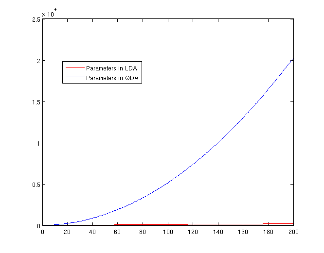
The Number of Parameters in LDA and QDA
Both LDA and QDA require us to estimate parameters. The more estimation we have to do, the less robust our classification algorithm will be.
LDA: Since we just need to compare the differences between one given class and remaining [math]\displaystyle{ \,K-1 }[/math] classes, totally, there are [math]\displaystyle{ \,K-1 }[/math] differences. For each of them, [math]\displaystyle{ \,a^{T}x+b }[/math] requires [math]\displaystyle{ \,d+1 }[/math] parameters. Therefore, there are [math]\displaystyle{ \,(K-1)\times(d+1) }[/math] parameters.
QDA: For each of the differences, [math]\displaystyle{ \,x^{T}ax + b^{T}x + c }[/math] requires [math]\displaystyle{ \frac{1}{2}(d+1)\times d + d + 1 = \frac{d(d+3)}{2}+1 }[/math] parameters. Therefore, there are [math]\displaystyle{ (K-1)(\frac{d(d+3)}{2}+1) }[/math] parameters.
Trick: Using LDA to do QDA
{{
Template:namespace detect
| type = style | image = | imageright = | style = | textstyle = | text = This article may require cleanup to meet Wikicoursenote's quality standards. The specific problem is: It must be noted that we don't do QDA with LDA and if we try QDA directly on this problem the resulting decision boundary will be different. Here we try to find a nonlinear boundary for a better possible boundary but it is different with general QDA method. We can call it nonlinear LDA. Please improve this article if you can. (October 2nd 2010) | small = | smallimage = | smallimageright = | smalltext = }} There is a trick that allows us to use the linear discriminant analysis (LDA) algorithm to generate as its output a quadratic function that can be used to classify data. This trick is similar to, but more primitive than, the Kernel trick that will be discussed later in the course.
Essentially, the trick involves adding one or more new features (i.e. new dimensions) that just contain our original data projected to that dimension. We then do LDA on our new higher-dimensional data. The answer provided by LDA can then be collapsed onto a lower dimension, giving us a quadratic answer.
Motivation
Why would we want to use LDA over QDA? In situations where we have fewer data points, LDA turns out to be more robust.
If we look back at the equations for LDA and QDA, we see that in LDA we must estimate [math]\displaystyle{ \,\mu_1 }[/math], [math]\displaystyle{ \,\mu_2 }[/math] and [math]\displaystyle{ \,\Sigma }[/math]. In QDA we must estimate all of those, plus another [math]\displaystyle{ \,\Sigma }[/math]; the extra [math]\displaystyle{ \,\frac{d(d-1)}{2} }[/math] estimations make QDA less robust with fewer data points.
Theoretically
Suppose we can estimate some vector [math]\displaystyle{ \underline{w}^T }[/math] such that
[math]\displaystyle{ y = \underline{w}^Tx }[/math]
where [math]\displaystyle{ \underline{w} }[/math] is a d-dimensional column vector, and [math]\displaystyle{ x\ \epsilon\ \mathbb{R}^d }[/math] (vector in d dimensions).
We also have a non-linear function [math]\displaystyle{ g(x) = y = x^Tvx + \underline{w}^Tx }[/math] that we cannot estimate.
Using our trick, we create two new vectors, [math]\displaystyle{ \,\underline{w}^* }[/math] and [math]\displaystyle{ \,x^* }[/math] such that:
[math]\displaystyle{ \underline{w}^{*T} = [w_1,w_2,...,w_d,v_1,v_2,...,v_d] }[/math]
and
[math]\displaystyle{ x^{*T} = [x_1,x_2,...,x_d,{x_1}^2,{x_2}^2,...,{x_d}^2] }[/math]
We can then estimate a new function, [math]\displaystyle{ g^*(x,x^2) = y^* = \underline{w}^{*T}x^* }[/math].
Note that we can do this for any [math]\displaystyle{ x }[/math] and in any dimension; we could extend a [math]\displaystyle{ D \times n }[/math] matrix to a quadratic dimension by appending another [math]\displaystyle{ D \times n }[/math] matrix with the original matrix squared, to a cubic dimension with the original matrix cubed, or even with a different function altogether, such as a [math]\displaystyle{ \,sin(x) }[/math] dimension.
By Example
Let's use our trick to do a quadratic analysis of the 2_3 data using LDA.
>> load 2_3;
>> [U, sample] = princomp(X');
>> sample = sample(:,1:2);
- We start off the same way, by using PCA to reduce the dimensionality of our data to 2.
>> X_star = zeros(400,4);
>> X_star(:,1:2) = sample(:,:);
>> for i=1:400
     for j=1:2
       X_star(i,j+2) = X_star(i,j)^2;
     end
   end
- This projects our sample into two more dimensions by squaring our initial two dimensional data set.
>> group = ones(400,1);
>> group(201:400) = 2;
>> [class, error, POSTERIOR, logp, coeff] = classify(X_star, X_star, group, 'linear');
>> sum (class==group)
ans =
   375
- We can now display our results.
>> k = coeff(1,2).const;
>> l = coeff(1,2).linear;
>> f = sprintf('0 = %g+%g*x+%g*y+%g*(x)^2+%g*(y)^2', k, l(1), l(2),l(3),l(4));
>> ezplot(f,[min(sample(:,1)), max(sample(:,1)), min(sample(:,2)), max(sample(:,2))]);
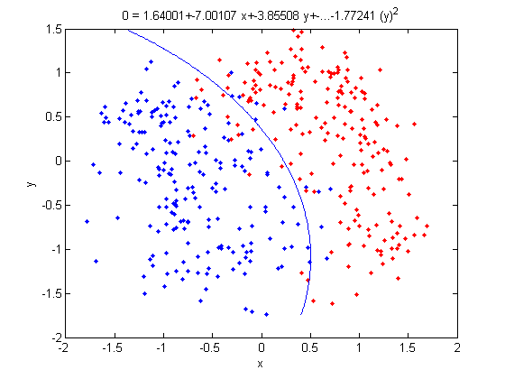
- Not only does LDA give us a better result than it did previously, it actually beats QDA, which only correctly classified 371 data points for this data set. Continuing this procedure by adding another two dimensions with [math]\displaystyle{ x^4 }[/math] (i.e. we set
X_star(i,j+2) = X_star(i,j)^4) we can correctly classify 376 points.
LDA and QDA in Matlab
We have examined the theory behind Linear Discriminant Analysis (LDA) and Quadratic Discriminant Analysis (QDA) above; how do we use these algorithms in practice? Matlab offers us a function called classify that allows us to perform LDA and QDA quickly and easily.
In class, we were shown an example of using LDA and QDA on the 2_3 data that is used in the first assignment. The code below reproduces that example, slightly modified, and explains each step.
>> load 2_3;
>> [U, sample] = princomp(X');
>> sample = sample(:,1:2);
- First, we do principal component analysis (PCA) on the 2_3 data to reduce the dimensionality of the original data from 64 dimensions to 2. Doing this makes it much easier to visualize the results of the LDA and QDA algorithms.
>> plot (sample(1:200,1), sample(1:200,2), 'b.');
>> hold on;
>> plot (sample(201:400,1), sample(201:400,2), 'r.');
- Recall that in the 2_3 data, the first 200 elements are images of the number two handwritten and the last 200 elements are images of the number three handwritten. This code sets up a plot of the data such that the points that represent a 2 are blue, while the points that represent a 3 are red.
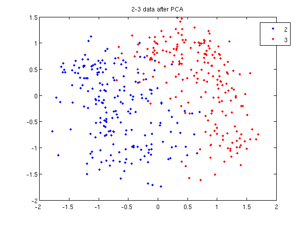
title and legend for information on adding the title and legend.- Before using
classifywe can set up a vector that contains the actual labels for our data, to train the classification algorithm. If we don't know the labels for the data, then the element in thegroupvector should be an empty string orNaN. (See grouping data for more information.)
>> group = ones(400,1);
>> group(201:400) = 2;
- We can now classify our data.
>> [class, error, POSTERIOR, logp, coeff] = classify(sample, sample, group, 'linear');
- The full details of this line can be examined in the Matlab help file linked above. What we care about are
class, which contains the labels that the algorithm thinks that each data point belongs to, andcoeff, which contains information about the line that algorithm created to separate the data into each class.
- We can see the efficacy of the algorithm by comparing
classtogroup.
>> sum (class==group)
ans =
   369
- This compares the value in
classto the value ingroup. The answer of 369 tells us that the algorithm correctly determined the class of the point 369 times, out of a possible 400 data points. This gives us an empirical error rate of 0.0775.
- We can see the line produced by LDA using
coeff.
>> k = coeff(1,2).const;
>> l = coeff(1,2).linear;
>> f = sprintf('0 = %g+%g*x+%g*y', k, l(1), l(2));
>> ezplot(f, [min(sample(:,1)), max(sample(:,1)), min(sample(:,2)), max(sample(:,2))]);
- Those familiar with the programming language C will find the
sprintfline refreshingly familiar; those with no exposure to C are directed to Matlab'ssprintfpage. Essentially, this code sets up the equation of the line in the form0 = a + bx + cy. We then use theezplotfunction to plot the line.
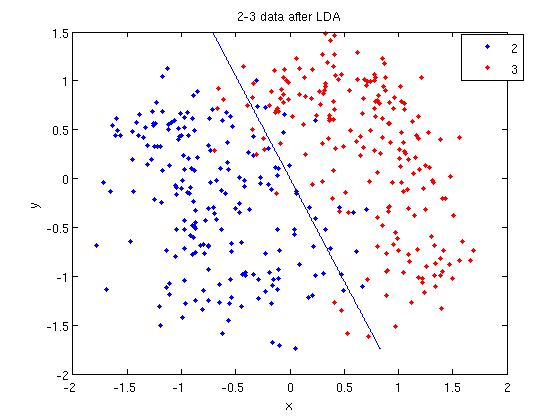
- Let's perform the same steps, except this time using QDA. The main difference with QDA is a slightly different call to
classify, and a more complicated procedure to plot the line.
>> [class, error, POSTERIOR, logp, coeff] = classify(sample, sample, group, 'quadratic');
>> sum (class==group)
ans =
   371
>> k = coeff(1,2).const;
>> l = coeff(1,2).linear;
>> q = coeff(1,2).quadratic;
>> f = sprintf('0 = %g+%g*x+%g*y+%g*x^2+%g*x.*y+%g*y^2', k, l(1), l(2), q(1,1), q(1,2)+q(2,1), q(2,2));
>> ezplot(f, [min(sample(:,1)), max(sample(:,1)), min(sample(:,2)), max(sample(:,2))]);
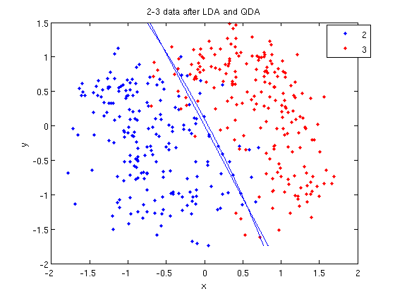
classify can also be used with other discriminant analysis algorithms. The steps laid out above would only need to be modified slightly for those algorithms.
Recall: An analysis of the function of princomp in matlab.
In our assignment 1, we have learnt that how to perform Principal Component Analysis using SVD method. In fact, the matlab offers us a function called princomp which can perform PCA conveniently. From the matlab help file on princomp, you can find the details about this function. But here we will analyze the code of the function of princomp() in matlab to find something different when comparing with SVD method. The following is the code of princomp and explanations to some emphasized steps.
   function [pc, score, latent, tsquare] = princomp(x);
   %   PRINCOMP Principal Component Analysis (centered and scaled data).
   %   [PC, SCORE, LATENT, TSQUARE] = PRINCOMP(X) takes a data matrix X and
   %   returns the principal components in PC, the so-called Z-scores in SC
   %   ORES, the eigenvalues of the covariance matrix of X in LATENT,
   %   and Hotelling's T-squared statistic for each data point in TSQUARE.
   %   Reference: J. Edward Jackson, A User's Guide to Principal Components
   %   John Wiley & Sons, Inc. 1991 pp. 1-25.
   %   B. Jones 3-17-94
   %   Copyright 1993-2002 The MathWorks, Inc.
   %   $Revision: 2.9 $  $Date: 2002/01/17 21:31:45 $
   [m,n] = size(x);       %  get the lengh of the rows and columns of matrix x.
   r = min(m-1,n);        %  max possible rank of X
   avg = mean(x);         %  the mean of every column of X
   centerx = (x - avg(ones(m,1),:));
                          %  centers X by subtracting off column means
   [U,latent,pc] = svd(centerx./sqrt(m-1),0);
                          %  "economy size" decomposition
   score = centerx*pc;
                          %  the representation of X in the principal component space
   if nargout < 3
      return;
    end
    latent = diag(latent).^2;
    if (r   latent = [latent(1:r); zeros(n-r,1)];
    score(:,r+1:end) = 0;
    end
    if nargout < 4
    return;
    end
    tmp = sqrt(diag(1./latent(1:r)))*score(:,1:r)';
    tsquare = sum(tmp.*tmp)';
From the above code, we should pay attention to the following aspects when comparing with SVD method:
First, Rows of [math]\displaystyle{ \,X }[/math] correspond to observations, columns to variables. When using princomp on 2_3 data in assignment 1, note that we take the transpose of [math]\displaystyle{ \,X }[/math].
 >> load 2_3;
 >> [U, score] = princomp(X');
Second, princomp centers X by subtracting off column means.
The third, when [math]\displaystyle{ \,X=UdV' }[/math], princomp uses [math]\displaystyle{ \,V }[/math] as coefficients for principal components, rather than [math]\displaystyle{ \,U }[/math].
The following is an example to perform PCA using princomp and SVD respectively to get the same results.
- SVD method
 >> load 2_3
 >> mn=mean(X,2);
 >> X1=X-repmat(mn,1,400);
 >> [s d v]=svd(X1');
 >> y=X1'*v;
- princomp
>>[U score]=princomp(X');
Then we can see that y=score, v=U.
useful resouces: LDA and QDA in Matlab[3],[4],[5]
Reference
1. Harry Zhang. The optimality of naive bayes. FLAIRS Conference. AAAI Press, 2004
2. Rich Caruana and Alexandru N. Mizil. An empirical comparison of supervised learning algorithms. In ICML ’06: Proceedings of the 23rd international conference on Machine learning, pages 161–168, New York, NY, USA, 2006, ACM.
3. The Elements of Statistical Learning: Data Mining, Inference, and Prediction, Second Edition, February 2009 Trevor Hastie, Robert Tibshirani, Jerome Friedman (3rd Edition is available)
Related links to LDA & QDA
LDA:[6]
Regularized linear discriminant analysis and its application in microarrays
MATHEMATICAL OPERATIONS OF LDA
Application in face recognition and in market
QDA:[8]
Principal Component Analysis
Principal Component Analysis (PCA) is a powerful technique for classification. It has applications in data visualization, data mining, reducing the dimensionality of a data set and etc. It is mostly used for data analysis and for making predictive models.
Rough definition
Keepings two important aspects of data analysis in mind:
- Reducing covariance in data
- Preserving information stored in data(Variance is a source of information)
PCA takes a sample of d - dimensional vectors and produces an orthogonal(zero covariance) set of d 'Principal Components'. The first Principal Component is the direction of greatest variance in the sample. The second principal component is the direction of second greatest variance (orthogonal to the first component), etc.
Then we can preserve most of the variance in the sample in a lower dimension by choosing the first k Principle Components and approximating the data in k - dimensional space, which is easier to analyze and plot.
Principal Components of handwritten digits
Suppose that we have a set of 103 images (28 by 23 pixels) of handwritten threes.
{{
Template:namespace detect
| type = style | image = | imageright = | style = | textstyle = | text = This article may require cleanup to meet Wikicoursenote's quality standards. The specific problem is: Would you please put appropriate pictures here. Please improve this article if you can. (3 October 2010) | small = | smallimage = | smallimageright = | smalltext = }}
We can represent each image as a vector of length 644 ([math]\displaystyle{ 644 = 23 \times 28 }[/math]). Then we can represent the entire data set as a 644 by 103 matrix, shown below. Each column represents one image (644 rows = 644 pixels).
Using PCA, we can approximate the data as the product of two smaller matrices, which I will call [math]\displaystyle{ V \in M_{644,2} }[/math] and [math]\displaystyle{ W \in M_{2,103} }[/math]. If we expand the matrix product then each image is approximated by a linear combination of the columns of V: [math]\displaystyle{ \hat{f}(\lambda) = \bar{x} + \lambda_1 v_1 + \lambda_2 v_2 }[/math], where [math]\displaystyle{ \lambda = [\lambda_1, \lambda_2]^T }[/math] is a column of W.
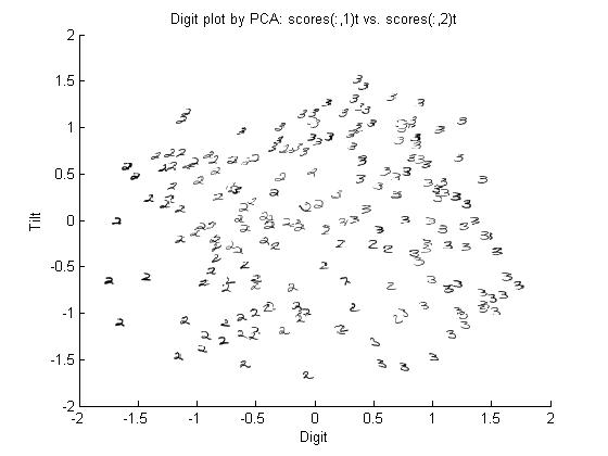
To demonstrate this process, we can compare the images of 2s and 3s. We will apply PCA to the data, and compare the images of the labeled data. This is an example in classifying.
Don't worry about the constant term for now. The point is that we can represent an image using just 2 coefficients instead of 644. Also notice that the coefficients correspond to features of the handwritten digits. The picture below shows the first two principal components for the set of handwritten threes.
{{
Template:namespace detect
| type = style | image = | imageright = | style = | textstyle = | text = This article may require cleanup to meet Wikicoursenote's quality standards. The specific problem is: Would you please put suitable picture here. Please improve this article if you can. (3 October 2010) | small = | smallimage = | smallimageright = | smalltext = }}
The first coefficient represents the width of the entire digit, and the second coefficient represents the slend of each digit handwritten.
Derivation of the first Principle Component
We want to find the direction of maximum variation. Let [math]\displaystyle{ \boldsymbol{w} }[/math] be an arbitrary direction, [math]\displaystyle{ \boldsymbol{x} }[/math] a data point and [math]\displaystyle{ \displaystyle u }[/math] the length of the projection of [math]\displaystyle{ \boldsymbol{x} }[/math] in direction [math]\displaystyle{ \boldsymbol{w} }[/math].
[math]\displaystyle{ \begin{align}
\textbf{w} &= [w_1, \ldots, w_D]^T \\
\textbf{x} &= [x_1, \ldots, x_D]^T \\
u &= \frac{\textbf{w}^T \textbf{x}}{\sqrt{\textbf{w}^T\textbf{w}}}
\end{align}
}[/math]
The direction [math]\displaystyle{ \textbf{w} }[/math] is the same as [math]\displaystyle{ c\textbf{w} }[/math] so without loss of generality,
[math]\displaystyle{
\begin{align}
|\textbf{w}| &= \sqrt{\textbf{w}^T\textbf{w}} = 1 \\
u &= \textbf{w}^T \textbf{x}
\end{align}
}[/math]
Let [math]\displaystyle{ x_1, \ldots, x_D }[/math] be random variables, then our goal is to maximize the variance of [math]\displaystyle{ u }[/math],
[math]\displaystyle{
\textrm{var}(u) = \textrm{var}(\textbf{w}^T \textbf{x}) = \textbf{w}^T \Sigma \textbf{w},
}[/math]
For a finite data set we replace the covariance matrix [math]\displaystyle{ \Sigma }[/math] by [math]\displaystyle{ s }[/math], the sample covariance matrix,
[math]\displaystyle{ \textrm{var}(u) = \textbf{w}^T s\textbf{w} }[/math]
is the variance of any vector [math]\displaystyle{ \displaystyle u }[/math], formed by the weight vector [math]\displaystyle{ \displaystyle w }[/math]. The first principal component is the vector that maximizes the variance,
[math]\displaystyle{
\textrm{PC} = \underset{\textbf{w}}{\operatorname{arg\,max}} \, \left( \operatorname{var}(u) \right) = \underset{\textbf{w}}{\operatorname{arg\,max}} \, \left( \textbf{w}^T s \textbf{w} \right)
}[/math]
where arg max denotes the value of [math]\displaystyle{ w }[/math] that maximizes the function. Our goal is to find the weights [math]\displaystyle{ \displaystyle w }[/math] that maximize this variability, subject to a constraint. The constraint in this case is fixing the size of the function, since this is a convex function that has no maximum value; however, we are interested only in the direction of the variability.
The problem then becomes,
[math]\displaystyle{
\underset{\textbf{w}}{\operatorname{max}} \, \left( \textbf{w}^T s \textbf{w} \right)
}[/math]
such that
[math]\displaystyle{ \textbf{w}^T \textbf{w} = 1 }[/math]
Notice,
[math]\displaystyle{
\textbf{w}^T s \textbf{w} \leq \| \textbf{w}^T s \textbf{w} \| \leq \| s \| \| \textbf{w} \| = \| s \|
}[/math]
Therefore the variance is bounded, so the maximum exists. We find the this maximum using the method of Lagrange multipliers.
Lagrange Multiplier
Before we can proceed, we must review Lagrange Multipliers.
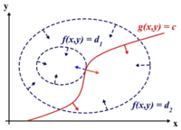
To find the maximum (or minimum) of a function [math]\displaystyle{ \displaystyle f(x,y) }[/math] subject to constraints [math]\displaystyle{ \displaystyle g(x,y) = 0 }[/math], we define a new variable [math]\displaystyle{ \displaystyle \lambda }[/math] called a Lagrange Multiplier and we form the Lagrangian,
[math]\displaystyle{ \displaystyle L(x,y,\lambda) = f(x,y) - \lambda g(x,y) }[/math]
If [math]\displaystyle{ \displaystyle (x^*,y^*) }[/math] is the max of [math]\displaystyle{ \displaystyle f(x,y) }[/math], there exists [math]\displaystyle{ \displaystyle \lambda^* }[/math] such that [math]\displaystyle{ \displaystyle (x^*,y^*,\lambda^*) }[/math] is a stationary point of [math]\displaystyle{ \displaystyle L }[/math] (partial derivatives are 0).
In addition [math]\displaystyle{ \displaystyle (x^*,y^*) }[/math] is a point in which functions [math]\displaystyle{ \displaystyle f }[/math] and [math]\displaystyle{ \displaystyle g }[/math] touch but do not cross. At this point, the tangents of [math]\displaystyle{ \displaystyle f }[/math] and [math]\displaystyle{ \displaystyle g }[/math] are parallel or gradients of [math]\displaystyle{ \displaystyle f }[/math] and [math]\displaystyle{ \displaystyle g }[/math] are parallel, such that:
[math]\displaystyle{ \displaystyle \nabla_{x,y } f = \lambda \nabla_{x,y } g }[/math]
where,
[math]\displaystyle{ \displaystyle \nabla_{x,y} f = (\frac{\partial f}{\partial x},\frac{\partial f}{\partial{y}}) \leftarrow }[/math] the gradient of [math]\displaystyle{ \, f }[/math]
[math]\displaystyle{ \displaystyle \nabla_{x,y} g = (\frac{\partial g}{\partial{x}},\frac{\partial{g}}{\partial{y}}) \leftarrow }[/math] the gradient of [math]\displaystyle{ \, g }[/math]
Example
Suppose we wish to maximise the function [math]\displaystyle{ \displaystyle f(x,y)=x-y }[/math] subject to the constraint [math]\displaystyle{ \displaystyle x^{2}+y^{2}=1 }[/math]. We can apply the Lagrange multiplier method on this example; the lagrangian is:
[math]\displaystyle{ \displaystyle L(x,y,\lambda) = x-y - \lambda (x^{2}+y^{2}-1) }[/math]
We want the partial derivatives equal to zero:
[math]\displaystyle{ \displaystyle \frac{\partial L}{\partial x}=1+2 \lambda x=0 }[/math]
[math]\displaystyle{ \displaystyle \frac{\partial L}{\partial y}=-1+2\lambda y=0 }[/math]
[math]\displaystyle{ \displaystyle \frac{\partial L}{\partial \lambda}=x^2+y^2-1 }[/math]
Solving the system we obtain 2 stationary points: [math]\displaystyle{ \displaystyle (\sqrt{2}/2,-\sqrt{2}/2) }[/math] and [math]\displaystyle{ \displaystyle (-\sqrt{2}/2,\sqrt{2}/2) }[/math]. In order to understand which one is the maximum, we just need to substitute it in [math]\displaystyle{ \displaystyle f(x,y) }[/math] and see which one as the biggest value. In this case the maximum is [math]\displaystyle{ \displaystyle (\sqrt{2}/2,-\sqrt{2}/2) }[/math].
Determining W
Back to the original problem, from the Lagrangian we obtain,
[math]\displaystyle{ \displaystyle L(\textbf{w},\lambda) = \textbf{w}^T S \textbf{w} - \lambda (\textbf{w}^T \textbf{w} - 1) }[/math]
If [math]\displaystyle{ \textbf{w}^T \textbf{w} }[/math] is a unit vector then the second part of the equation is 0.
If [math]\displaystyle{ \textbf{w}^T \textbf{w} }[/math] is not a unit vector the the second part of the equation increases. Thus decreasing overall [math]\displaystyle{ \displaystyle L(\textbf{w},\lambda) }[/math]. Maximization happens when [math]\displaystyle{ \textbf{w}^T \textbf{w} =1 }[/math]
(Note that to take the derivative with respect to w below, [math]\displaystyle{ \textbf{w}^T S \textbf{w} }[/math] can be thought of as a quadratic function of w, hence the 2sw below. For more matrix derivatives, see section 2 of the Matrix Cookbook)
Taking the derivative with respect to w, we get:
[math]\displaystyle{ \displaystyle \frac{\partial L}{\partial \textbf{w}} = 2S\textbf{w} - 2\lambda\textbf{w} }[/math]
Set [math]\displaystyle{ \displaystyle \frac{\partial L}{\partial \textbf{w}} = 0 }[/math], we get
[math]\displaystyle{ \displaystyle S\textbf{w}^* = \lambda^*\textbf{w}^* }[/math]
From the eigenvalue equation [math]\displaystyle{ \, \textbf{w}^* }[/math] is an eigenvector of S and [math]\displaystyle{ \, \lambda^* }[/math] is the corresponding eigenvalue of S. If we substitute [math]\displaystyle{ \displaystyle\textbf{w}^* }[/math] in [math]\displaystyle{ \displaystyle \textbf{w}^T S\textbf{w} }[/math] we obtain,
[math]\displaystyle{ \displaystyle\textbf{w}^{*T} S\textbf{w}^* = \textbf{w}^{*T} \lambda^* \textbf{w}^* = \lambda^* \textbf{w}^{*T} \textbf{w}^* = \lambda^* }[/math]
In order to maximize the objective function we choose the eigenvector corresponding to the largest eigenvalue. We choose the first PC, u1 to have the maximum variance
(i.e. capturing as much variability in in [math]\displaystyle{ \displaystyle x_1, x_2,...,x_D }[/math] as possible.) Subsequent principal components will take up successively smaller parts of the total variability.
D dimensional data will have D eigenvectors
[math]\displaystyle{ \lambda_1 \geq \lambda_2 \geq ... \geq \lambda_D }[/math] where each [math]\displaystyle{ \, \lambda_i }[/math] represents the amount of variation in direction [math]\displaystyle{ \, i }[/math]
so that
[math]\displaystyle{ Var(u_1) \geq Var(u_2) \geq ... \geq Var(u_D) }[/math]
Note that the Principal Components decompose the total variance in the data:
[math]\displaystyle{ \displaystyle \sum_{i = 1}^D Var(u_i) = \sum_{i = 1}^D \lambda_i = Tr(S) = \sum_{i = 1}^D Var(x_i) }[/math]
i.e. the sum of variations in all directions is the variation in the whole data
Example from class
We apply PCA to the noise data, making the assumption that the intrinsic dimensionality of the data is 10. We now try to compute the reconstructed images using the top 10 eigenvectors and plot the original and reconstructed images
The Matlab code is as follows:
 load noisy
 who
 size(X)
 imagesc(reshape(X(:,1),20,28)')
 colormap gray
 imagesc(reshape(X(:,1),20,28)')
 [u s v] = svd(X);
 xHat = u(:,1:10)*s(1:10,1:10)*v(:,1:10)'; % use ten principal components
 figure
 imagesc(reshape(xHat(:,1000),20,28)') % here '1000' can be changed to different values, e.g. 105, 500, etc.
 colormap gray
Running the above code gives us 2 images - the first one represents the noisy data - we can barely make out the face
The second one is the denoised image
-
"Noisy Face"
-
"De-noised Face"
As you can clearly see, more features can be distinguished from the picture of the de-noised face compared to the picture of the noisy face. If we took more principal components, at first the image would improve since the intrinsic dimensionality is probably more than 10. But if you include all the components you get the noisy image, so not all of the principal components improve the image. In general, it is difficult to choose the optimal number of components.
Application of PCA - Feature Abstraction
One of the applications of PCA is to group similar data (e.g. images). There are generally two methods to do this. We can classify the data (i.e. give each data a label and compare different types of data) or cluster (i.e. do not label the data and compare output for classes).
Generally speaking, we can do this with the entire data set (if we have an 8X8 picture, we can use all 64 pixels). However, this is hard, and it is easier to use the reduced data and features of the data.
General PCA Algorithm
The PCA Algorithm is summarized in the following slide (taken from the Lecture Slides).
Algorithm
Recover basis: Calculate [math]\displaystyle{ XX^T =\Sigma_{i=1}^{T}= x_i x_{i}^{T} }[/math] and let [math]\displaystyle{ U= }[/math] eigenvectors of [math]\displaystyle{ X X^T }[/math] corresponding to the top [math]\displaystyle{ d }[/math] eigenvalues.
Encoding training data: Let [math]\displaystyle{ Y=U^TX }[/math] where [math]\displaystyle{ Y }[/math] is a [math]\displaystyle{ d \times t }[/math] matrix of encoding of the original data.
Reconstructing training data: [math]\displaystyle{ \hat{X}= UY=UU^TX }[/math].
Encode set example: [math]\displaystyle{ y=U^T x }[/math] where [math]\displaystyle{ y }[/math] is a [math]\displaystyle{ d- }[/math]dimentional encoding of [math]\displaystyle{ x }[/math].
Reconstruct test example: [math]\displaystyle{ \hat{x}= Uy=UU^Tx }[/math].
Other Notes:
- The mean of the data(X) must be 0. This means we may have to preprocess the data by subtracting off the mean(see detailsPCA in Wikipedia.)
- Encoding the data means that we are projecting the data onto a lower dimensional subspace by taking the inner product. Encoding: [math]\displaystyle{ X_{D\times n} \longrightarrow Y_{d\times n} }[/math] using mapping [math]\displaystyle{ \, U^T X_{d \times n} }[/math].
- When we reconstruct the training set, we are only using the top d dimensions.This will eliminate the dimensions that have lower variance (e.g. noise). Reconstructing: [math]\displaystyle{ \hat{X}_{D\times n}\longleftarrow Y_{d \times n} }[/math] using mapping [math]\displaystyle{ \, UY_{D \times n} }[/math].
- We can compare the reconstructed test sample to the reconstructed training sample to classify the new data.
Fisher's Linear Discriminant Analysis (FDA) October 5, 2010
Lecture Summary
In This lecture introduces Fisher's Discriminant Analysis method. While discussing the goals specified by Fisher for his analysis. Then proceeding by mathematical formulation of these goals. The lecture summarizes the topic with General solution that satisfies these goals.
Fisher's Discriminant Analysis (FDA), also known as Fisher's Linear Discriminant Analysis (LDA) in some sources, is a classical feature extraction technique. It was originally described in 1936 by Sir Ronald Aylmer Fisher, an English statistician and eugenicist who has been described as one of the founders of modern statistical science. His original paper describing FDA can be found here; a Wikipedia article summarizing the algorithm can be found here.
Contrasting FDA with PCA
Similar to PCA, the goal of FDA is to project the data in a lower dimension. The difference is that we we are not interested in maximizing variances. Rather our goal is to find a direction that is useful for classifying the data (i.e. in this case, we are looking for direction representative of a particular characteristic e.g. glasses vs. no-glasses).
The number of dimensions that we want to reduce the data to, depends on the number of classes:
For a 2 class problem, we want to reduce the data to one dimension (a line), [math]\displaystyle{ \displaystyle Z \in \mathbb{R}^{1} }[/math]
Generally, for a k class problem, we want k-1 dimensions, [math]\displaystyle{ \displaystyle Z \in \mathbb{R}^{k-1} }[/math]
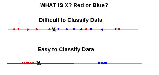
As we will see from our objective function, we want to maximize the separation of the classes and to minimize the within variance of each class. That is, our ideal situation is that the individual classes are as far away from each other as possible, but the data within each class is close together (i.e. collapse to a single point).
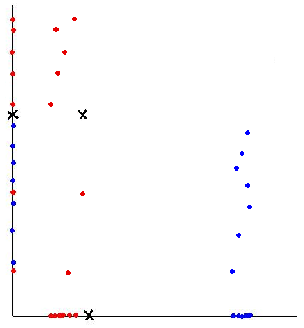
The following diagram summarizes this goal.
In fact, the two examples above may represent the same data projected on two different lines.
Two-class problem
In the two-class problem, we have the pre-knowledge that data points belong to two classes. Intuitively speaking points of each class form a cloud around the mean of the class, with each class having possibly different size. To be able to separate the two classes we must determine the class whose mean is closest to a given point while also accounting for the different size of each class, which is represented by the covariance of each class.
Assume [math]\displaystyle{ \underline{\mu_{1}}=\frac{1}{n_{1}}\displaystyle\sum_{i:y_{i}=1}\underline{x_{i}} }[/math] and [math]\displaystyle{ \displaystyle\Sigma_{1} }[/math], represent the mean and covariance of the 1st class, and [math]\displaystyle{ \underline{\mu_{2}}=\frac{1}{n_{2}}\displaystyle\sum_{i:y_{i}=2}\underline{x_{i}} }[/math] and [math]\displaystyle{ \displaystyle\Sigma_{2} }[/math] represent the mean and covariance of the 2nd class. We have to find a transformation which satisfies the following goals:
1.To make the means of these two classes as far apart as possible
- In other words, the goal is to maximize the distance after projection between class 1 and class 2. This can be done by maximizing the distance between the means of the classes after projection. When projecting the data points to a one-dimensional space, all points will be projected to a single line; the line we seek is the one with the direction that achieves maximum separation of classes upon projetion. If the original points are [math]\displaystyle{ \underline{x_{i}} \in \mathbb{R}^{d} }[/math]and the projected points are [math]\displaystyle{ \underline{w}^T \underline{x_{i}} }[/math] then the mean of the projected points will be [math]\displaystyle{ \underline{w}^T \underline{\mu_{1}} }[/math] and [math]\displaystyle{ \underline{w}^T \underline{\mu_{2}} }[/math] for class 1 and class 2 respectively. The goal now becomes to maximize the Euclidean distance between projected means, [math]\displaystyle{ (\underline{w}^T\underline{\mu_{1}}-\underline{w}^T\underline{\mu_{2}})^T (\underline{w}^T\underline{\mu_{1}}-\underline{w}^T\underline{\mu_{2}}) }[/math]. The steps of this maximization are given below.
2.We want to collapse all data points of each class to a single point, i.e., minimize the covariance within classes
- Notice that the variance of the projected classes 1 and 2 are given by [math]\displaystyle{ \underline{w}^T\Sigma_{1}\underline{w} }[/math] and [math]\displaystyle{ \underline{w}^T\Sigma_{2}\underline{w} }[/math]. The second goal is to minimize the sum of these two covariances.
As is demonstrated below, both of these goals can be accomplished simultaneously.
Original points are [math]\displaystyle{ \underline{x_{i}} \in \mathbb{R}^{d} }[/math]
[math]\displaystyle{ \ \{ \underline x_1 \underline x_2 \cdot \cdot \cdot \underline x_n \} }[/math]
Projected points are [math]\displaystyle{ \underline{z_{i}} \in \mathbb{R}^{1} }[/math] with [math]\displaystyle{ \underline{z_{i}} = \underline{w}^T \cdot\underline{x_{i}} }[/math] [math]\displaystyle{ \ z_i }[/math] is a sclar
FDA Goals
Fisher has defined two goals by which the quality of discrimination is maximized.
1. Maximum Separation
[math]\displaystyle{ \displaystyle \min (w^T\sum_1w) }[/math]
[math]\displaystyle{ \displaystyle \min (w^T\sum_2w) }[/math]
and this problem reduces to [math]\displaystyle{ \displaystyle \min (w^T(\sum_1 + \sum_2)w) }[/math]
(where [math]\displaystyle{ \displaystyle \sum_1 and \sum_2 }[/math] are the covariance matrices for the 1st and 2nd class of data respectively)
Let [math]\displaystyle{ \displaystyle \ s_w=\sum_1 + \sum_2 }[/math] be the within classes covariance. Then, this problem can be rewritten as [math]\displaystyle{ \displaystyle \min (w^Ts_ww) }[/math]
2. Maximize the distance between the means of the projected data
The optimization problem we want to solve is,
[math]\displaystyle{ \displaystyle \max (w^T \mu_1 - w^T \mu_2)^2, }[/math]
[math]\displaystyle{ \begin{align} (w^T \mu_1 - w^T \mu_2)^2 &= (w^T \mu_1 - w^T \mu_2)^T(w^T \mu_1 - w^T \mu_2)\\
&= (\mu_1^Tw - \mu_2^Tw^T)(w^T \mu_1 - w^T \mu_2)\\
&= (\mu_1^T - \mu_2^T)ww^T(\mu_1 - \mu_2) \end{align} }[/math]
which is a scalar. Therefore,
[math]\displaystyle{ \displaystyle = tr[(\mu_1^T - \mu_2^T)ww^T(\mu_1 - \mu_2)] }[/math]
[math]\displaystyle{ \displaystyle = tr[w^T(\mu_1 - \mu_2)(\mu_1 - \mu_2)^Tw] }[/math]
(using the property of [math]\displaystyle{ \displaystyle tr[ABC] = tr[CAB] = tr[BCA] }[/math]
[math]\displaystyle{ \displaystyle = w^T(\mu_1 - \mu_2)(\mu_1 - \mu_2)^Tw }[/math]
Thus our original problem equivalent can be written as,
[math]\displaystyle{ \displaystyle \max (w^T \mu_1 - w^T \mu_2)^2 = \displaystyle \max (w^T(\mu_1 - \mu_2)(\mu_1 - \mu_2)^Tw) }[/math]
For a two class problem the between class variance is,
[math]\displaystyle{ \displaystyle \ s_B=(\mu_1 - \mu_2)(\mu_1 - \mu_2)^T }[/math]
Then this problem can be rewritten as,
[math]\displaystyle{ \displaystyle \max (w^Ts_Bw) }[/math]
Objective Function
We want an objective function which satisifies both of the goals outlined above (at the same time).
- [math]\displaystyle{ \displaystyle \min (w^T(\sum_1 + \sum_2)w) }[/math] or [math]\displaystyle{ \displaystyle \min (w^Ts_ww) }[/math]
- [math]\displaystyle{ \displaystyle \max (w^T(\mu_1 - \mu_2)(\mu_1 - \mu_2)^Tw) }[/math] or [math]\displaystyle{ \displaystyle \max (w^Ts_Bw) }[/math]
We take the ratio of the two -- we wish to maximize
[math]\displaystyle{ \displaystyle \frac{(w^T(\mu_1 - \mu_2)(\mu_1 - \mu_2)^Tw)} {(w^T(\sum_1 + \sum_2)w)} }[/math]
or equivalently,
[math]\displaystyle{ \displaystyle \max \frac{(w^Ts_Bw)}{(w^Ts_ww)} }[/math]
This is a very famous problem which is called "the generalized eigenvector problem". We can solve this using Lagrange Multipliers. Since W is a directional vector, we do not care about the size of W. Therefore we solve a problem similar to that in PCA,
[math]\displaystyle{ \displaystyle \max (w^Ts_Bw) }[/math]
subject to [math]\displaystyle{ \displaystyle (w^Ts_Ww=1) }[/math] (In the general optimization form, 1 is replaced with constant b)
where [math]\displaystyle{ s_B }[/math] is the covariance matrix between classes and [math]\displaystyle{ s_w }[/math] is the covariance matrix within classes.
We solve the following Lagrange Multiplier problem,
[math]\displaystyle{ \displaystyle L(w,\lambda) = w^Ts_Bw - \lambda (w^Ts_Ww -1) }[/math]
So, we have a Partial solution to: [math]\displaystyle{ \displaystyle (w^Ts_Bw) - \lambda \cdot [(w^Ts_ww)-1] }[/math]
- The optimal solution for w is the eigenvector of [math]\displaystyle{ \displaystyle s_w^{-1}s_B }[/math] corresponding to the largest eigenvalue;
- For a k class problem, we will take the eigenvectors corresponding to the (k-1) highest eigenvalues.
- In the case of two-class problem, the optimal solution for w can be simplfied, such that: [math]\displaystyle{ \displaystyle w \propto s_w^{-1}(\mu_2 - \mu_1) }[/math]
FDA Using Matlab
We see now an application of the theory that we just introduced. Using Matlab, we find the principal components and the projection by Fisher Discriminant Analysis of two Bivariate normal distributions to show the difference between the two methods.
      %First of all, we generate the two data set:
      X1 = mvnrnd([1,1],[1 1.5; 1.5 3], 300)
      %In this case: mu_1=[1;1]; Sigma_1=[1 1.5; 1.5 3], where mu and sigma are the mean and covariance matrix.
      X2 = mvnrnd([5,3],[1 1.5; 1.5 3], 300)
      %Here mu_2=[5;3] and Sigma_2=[1 1.5; 1.5 3]
      %The plot of the two distributions is:
      %We compute the principal components:
      X=[X1,X2]
      X=X'
      [coefs, scores]=princomp(X');
      coefs(:,1)    %first principal component
      coefs(:,1)

      ans =
      0.76355476446932
      0.64574307712603

      plot([0 coefs(1,1)], [0 coefs(2,1)],'b')
      plot([0 coefs(1,1)]*10, [0 coefs(2,1)]*10,'r')
      sw=2*[1 1.5;1.5 3]   % sw=Sigma1+Sigma2=2*Sigma1
      w=sw\[4; 2]       % calculate s_w^{-1}(mu2 - mu1)
      plot ([0 w(1)], [0 w(2)],'g')
      %We now make the projection:
      Xf=w'*X
      figure
      plot(Xf(1:300),1,'ob') %In this case, since it's a one dimension data, the plot is "Data Vs Indexes"
      hold on
      plot(Xf(301:600),1,'or')
      %We see that in the above picture that there is no overlapping
      Xp=coefs(:,1)'*X
      figure
      plot(Xp(1:300),1,'b')
      hold on
      plot(Xp(301:600),2,'or')
%In this case there is an overlapping since we project the first principal component on [Xp=coefs(:,1)'*X]
- Pages with broken file links
- Articles needing cleanup from 29 September 2010
- Articles with invalid date parameter in template
- All pages needing cleanup
- Articles needing cleanup from October 2nd 2010
- Articles needing cleanup from September 2010
- Articles needing cleanup from October 2010
- Articles needing cleanup from 3 October 2010
