Self-Supervised Learning of Pretext-Invariant Representations: Difference between revisions
| Line 87: | Line 87: | ||
===Does PIRL learn invariant representations?=== | ===Does PIRL learn invariant representations?=== | ||
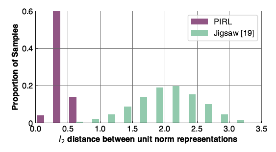
In order to show that | In order to show that the image representations obtained using PIRL are invariant, | ||
[[File: SSL_7.PNG | 800px | center]] | [[File: SSL_7.PNG | 800px | center]] | ||
Revision as of 16:44, 29 November 2020
Presented by
Sina Farsangi
Introduction
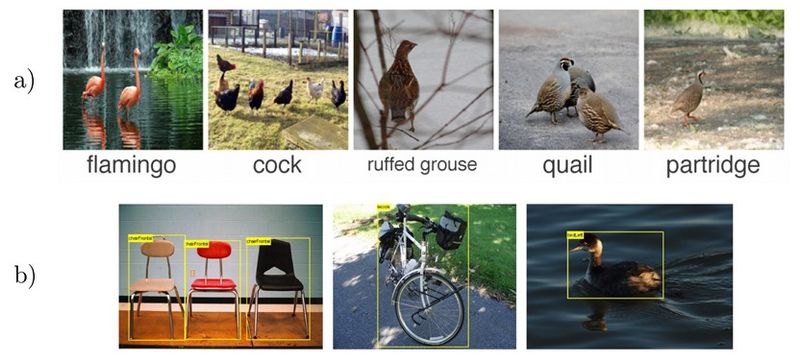
Modern image recognition and object detection systems find image representations using a large number data with pre-defined semantic annotation. Some examples of these annotations are class labels and bonding boxes as shown in Figure 1. For finding representations using pre-defined semantic annotations, there is a need for large number of labeled data which is not the case in all scenarios. Also, these systems usually learn features that are specific for a particular type of class and not necessarily semantically meaningful features that can help to generalize to other domains and classes. In other words, pre-defined semantic annotations scale poorly to the long scale of visual concepts[1]. Therefore, there has been a big interest in the community to find image representations that are more visually meaningful and can help in several tasks such as image recognition and object detection. One of the fast growing areas of research that tries to address this problem is Self-Supervised Learning. Self-Supervised Learning tries to learn deep models that find image representations from the pixels themselves rather than using pre-defined semantic annotated data. As we will show, there is no need for using class labels [1] or bounding boxes [2] in self-supervised learning.
Self-Supervised Learning is often done using a set of tasks called Pretext tasks. During these tasks, a transformation [math]\displaystyle{ \tau }[/math] is applied to unlabeled images [math]\displaystyle{ I }[/math] to obtain a set of transformed images, [math]\displaystyle{ I^{t} }[/math]. Then, a deep neural network, [math]\displaystyle{ \phi(\theta) }[/math], is trained to predict the transformation characteristic. Several Pretext Tasks exist based on the type of used transformation. Two of the most used pretext tasks are rotations and jigsaw puzzle [3,4,5]. As shown in Figure 2, in the rotation task, unlabeled images, [math]\displaystyle{ }[/math] are rotated by random degrees (0,90,180,270) and the deep network learns to predict the rotation degree. Also, in jigsaw task which is more complicated than rotation task, unlabeled images are cropped into 9 patches and then, the image is perturbed by randomly permuting the nine patches. Then, a deep network is trained to predict the permutation of the patches in the perturbed image.

Although the proposed pretext tasks have obtained promising results, they have the disadvantage of being covariant to the applied transformation. In other words, as deep networks are trained to predict transformations characteristics, they will also learn representations that will vary based on the applied transformation. By intuition, we would like to obtain representations the are common between the original images and the transformed ones. This idea is supported by the fact that humans are able to recognize these transformed images. This hints us to try to develop a method that obtains image representations that are common between the original and transformed images, in other words, image representations that are transformation invariant. The summarized paper tries to address this problem by introducing Pretext Invariant Representation Learning (PIRL) that learns to obtain self-supervised image representations that as opposed to Pretext tasks are transformation invariant and therefore, more semantically meaningful. The performance of the proposed method is evaluated on several self-supervision learning benchmarks. The results show that the PIRL introduces a new state-of-the-art method in Self-Supervised Learning by learning transformation invariant representations.
Problem Formulation and Methodology
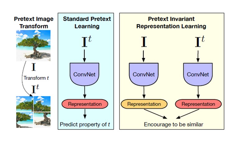
An overview of the proposed method and a comparison with Pretext Tasks are shown in Figure 3. For a given image ,[math]\displaystyle{ I }[/math], in the Dataset of unlabeled images, [math]\displaystyle{ D=\{{I_1,I_2,...,I_{|D|}}\} }[/math], a transformation [math]\displaystyle{ \tau }[/math] is applied:
\begin{align} \tag{1} \label{eqn:1} I^t=\tau(I) \end{align}
Where [math]\displaystyle{ I^t }[/math] is the transformed image. We would like to train a convolutional neural network, [math]\displaystyle{ \phi(\theta) }[/math], that constructs image representations [math]\displaystyle{ v_{I}=\phi_{\theta}(I) }[/math]. Pretext Task based methods learn to predict transformation characteristics, [math]\displaystyle{ z(t) }[/math], by minimizing a transformation covariant loss function in the form of:
\begin{align} \tag{2} \label{eqn:2} l_{\text{cov}}(\theta,D)=\frac{1}{|D|} \sum_{I \in {D}}^{} L(v_I,z(t) \end{align}
As it can be seen, the loss function covaries with the applied transformation and therefore, the obtained representations may not be semantically meaningful. PIRL tries to solve for this problem as shown in Figure 3. The original and transformed images are passed through two parallel convolutional neural networks to obtain two set of representations, [math]\displaystyle{ v(I) }[/math] and [math]\displaystyle{ v(I^t) }[/math]. Then, a contrastive loss function is defined to ensure that the representations of the original and transformed images are similar to each other. The transformation invariant loss function can be defined as:
\begin{align} \tag{3} \label{eqn:3} l_{\text{inv}}(\theta,D)=\frac{1}{|D|} \sum_{I \in {D}}^{} L(v_I,v_{I^t}) \end{align}
Where L is a contrastive loss based on Noise Contrastive Estimators (NCE). The NCE function can be shown as below:
\begin{align} \tag{4} \label{eqn:4} h(v_I,v_{I^t})=\frac{\exp \biggl( \frac{s(v_I,v_{I^t}}{\tau}) \biggr)}{\exp \biggl(\frac{s(v_I,v_{I^t}}{\tau} \biggr) + \sum_{I^{'} \in D_N}^{} \exp \biggl( \frac{s(v_{I^t},v_{I^{'}}}{\tau}) \biggr)} \end{align}
where [math]\displaystyle{ s(.,.) }[/math] is the cosine similarity function and [math]\displaystyle{ \tau }[/math] is the temperature parameter that is usually set to 0.07. Also, a set of N images are chosen randomly from dataset where [math]\displaystyle{ I^{'}\neq I }[/math]. These images are used in the loss in order to ensure their representation dissimilarity with transformed image representations. Also, during model implementation, two heads (few additional deep layers) , [math]\displaystyle{ f }[/math] and [math]\displaystyle{ g }[/math], are applied on top of [math]\displaystyle{ v(I) }[/math] and [math]\displaystyle{ v(I^t) }[/math]. Using the NCE formulation, the contrastive loss can be written as:
\begin{align} \tag{5} \label{eqn:5} L_{\text{NCE}}(I,I^{t})=-\text{log}[h(f(v_I),g(v_{I^t}))]-\sum_{I^{'}\in D_N}^{} \text{log}[1-h(g(v_{I^t}),f(v_{I^{'}}))] \end{align}
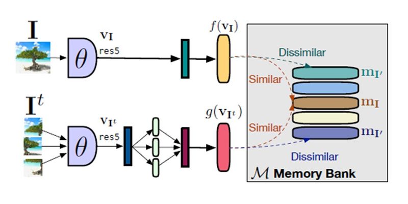
Although the formulation looks complicated, the take out here is that by minimizing the NCE based loss function, the similarity between the original and transformed image representations, [math]\displaystyle{ v(I) }[/math] and [math]\displaystyle{ v(I^t) }[/math] , increases and at the same time the dissimilarity between [math]\displaystyle{ v(I^t) }[/math] and negative images representations, [math]\displaystyle{ v(I^{'}) }[/math], are increased. During training a memory bank [], [math]\displaystyle{ m_I }[/math], of dataset image representations are used to access the representations of the dataset images including the negative images. The proposed PIRL model is shown in Figure (4). Finally, the contrastive loss in equation (5) does not take into account the dissimilarity between the original image representations, [math]\displaystyle{ v(I) }[/math], and the negative image representations, [math]\displaystyle{ v(I^{'}) }[/math]. By taking this into account and using the memory bank, the final constrastive loss function is obtained as:
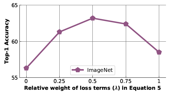
\begin{align} \tag{6} \label{eqn:6} L(I,I^{t})=\lambda L_{\text{NCE}}(m_I,g(v_{I^t})) + (1-\lambda)L_{\text{NCE}}(m_I,f(v_{I})) \end{align} Where [math]\displaystyle{ \lambda }[/math] is a hyperparameter that determines the weight of each of NCE losses. The default value for this parameter is 0.5. In the next section, experimental results are shown using the proposed PIRL model.
Experimental Results
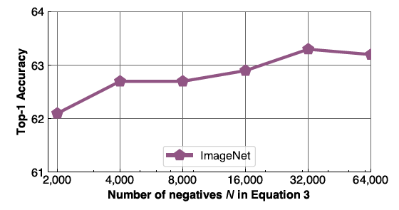
In this section, the quality of image representations obtained from PIRL Self-Supervised Learning is evaluated by comparing its performance to other Self-Supervised Learning methods on image recognition and object detection tasks. For the experiments, a ResNet50 model is trained using PIRL and other methods by using 1.28M randomly sampled images from Imagenet dataset. Also, the number of negative images used for PIRL in N=32000.
Object Detection
For object detection, a Faster R-CNN[] model is used with a ResNet-50 backbone which is pre-trained using PIRL and other Self-Supervised methods. Then, the pre-trained model weights are used as initial weights for the Faster-RCNN model backbone during training on VOC07+12 dataset. The result of object detection using PIRL is shown in Figure (5) and it is compared to other methods. It can be seen that PIRL not only outperforms other self-supervised based methods, for the first time it outperforms Supervised Pretraining on object detection.
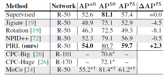
Image Classification with linear models
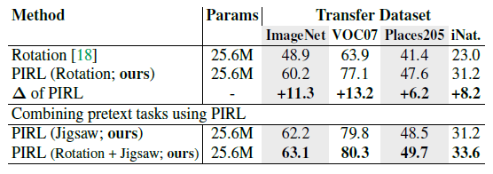
In the next experiment, the performance of the PIRL is evaluated on image classification using four different datasets. For this experiment, the ResNet-50 pretrained model is fixed and used as an image feature extractor. Then, a linear classifier is trained on fixed image representations. The results are shown in Figure (6). The results show that while PIRL substantially outperforms other Self-Supervised Learning methods, it still falls behinds supervised pretrained learning.
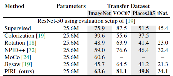
Overall, the results show that PIRL performs best among different Self-Supervised Learning methods. Even, it is able to perform better than Supervised Learning Pretrained model on object detection. This is because PIRL learns representations that are invariant to the applied transformations which results in more semantically meaningful and richer visual features. In the next section, some analysis on PIRL is presented.
Analysis
Does PIRL learn invariant representations?
In order to show that the image representations obtained using PIRL are invariant,
Conclusion
Critiques
Source Code
References
[1]