Influenza Forecasting Framework based on Gaussian Processes: Difference between revisions
| Line 43: | Line 43: | ||
<div style="text-align:center;"> [[File:GPRegression.png|600px]] </div> | <div style="text-align:center;"> [[File:GPRegression.png|600px]] </div> | ||
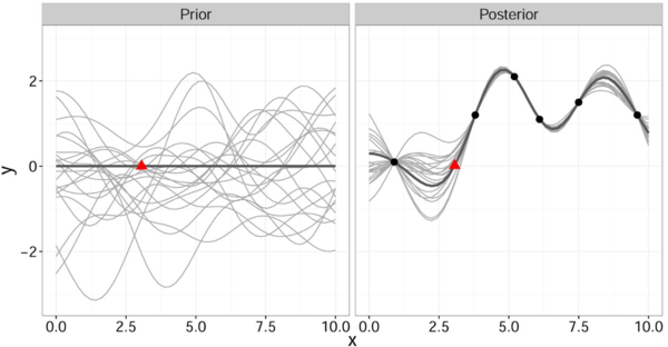
<div align="center">'''Figure 1''': Select the functions from your joint prior distribution (left, grey curves) with mean <math>0</math> (left, bold line) that agree with the observed data points (right, black bullets). These form your posterior distribution (right, grey curves) with mean <math>\mu(\mathbf{x})</math> (right, bold line). Red triangle helps compare the two images (location marker). </div> | <div align="center">'''Figure 1. Gaussian process regression''': Select the functions from your joint prior distribution (left, grey curves) with mean <math>0</math> (left, bold line) that agree with the observed data points (right, black bullets). These form your posterior distribution (right, grey curves) with mean <math>\mu(\mathbf{x})</math> (right, bold line). Red triangle helps compare the two images (location marker). </div> | ||
== Data-set Description == | == Data-set Description == | ||
Revision as of 01:29, 16 November 2020
Abstract
This paper presents a novel framework for seasonal epidemic forecasting using Gaussian process regression. Resulting retrospective forecasts, trained on a subset of the publicly available CDC influenza-like-illness (ILI) data-set, outperformed four state-of-the-art models when compared using the official CDC scoring rule (log-score).
Background
Each year, the seasonal influenza epidemic affects public health at a massive scale, resulting in 38 million cases, 400 000 hospitalizations, and 22 000 deaths in the United States in 2019/20 alone (cite CDC). Given this, reliable forecasts of future influenza development are invaluable, because they allow for improved public health policies and informed resource development and allocation.
Related Work
Given the value of epidemic forecasts, the CDC regularly publishes ILI data and has funded a seasonal ILI forecasting challenge. This challenge has lead to four state of the art models in the field; MSS, a physical susceptible-infected-recovered model with assumed linear noise; SARIMA, a framework based on seasonal auto-regressive moving average models; and LinEns, an ensemble of three linear regression models.
Motivation
It has been shown that LinEns forecasts outperform the other frameworks on the ILI data-set. However, this framework assumes a deterministic relationship between the epidemic week and its case count, which does not reflect the stochastic nature of the trend. Therefore, it is natural to ask whether a similar framework that assumes a stochastic relationship between these variables would provide better performance. This motivated the development of the proposed Gaussian process regression framework, and the subsequent performance comparison to the benchmark models.
Gaussian Process Regression
Consider the following set up: let [math]\displaystyle{ X = [\mathbf{x}_1,\ldots,\mathbf{x}_n] }[/math] [math]\displaystyle{ (d\times n) }[/math] be your training data, [math]\displaystyle{ \mathbf{y} = [y_1,y_2,\ldots,y_n]^T }[/math] be your noisy observations where [math]\displaystyle{ y_i = f(\mathbf{x}_i) + \epsilon_i }[/math], [math]\displaystyle{ (\epsilon_i:i = 1,\ldots,n) }[/math] i.i.d. [math]\displaystyle{ \sim \mathcal{N}(0,{\sigma}^2) }[/math], and [math]\displaystyle{ f }[/math] is the trend we are trying to model (by [math]\displaystyle{ \hat{f} }[/math]). Let [math]\displaystyle{ \mathbf{x}^* }[/math] [math]\displaystyle{ (d\times 1) }[/math] be your test data point, and [math]\displaystyle{ \hat{y} = \hat{f}(\mathbf{x}^*) }[/math] be your predicted outcome.
Instead of assuming a deterministic form of [math]\displaystyle{ f }[/math], and thus of [math]\displaystyle{ \mathbf{y} }[/math] and [math]\displaystyle{ \hat{y} }[/math] (as classical linear regression would, for example), Gaussian process regression assumes [math]\displaystyle{ f }[/math] is stochastic. More precisely, [math]\displaystyle{ \mathbf{y} }[/math] and [math]\displaystyle{ \hat{y} }[/math] are assumed to have a joint prior distribution. Indeed, we have
$$ (\mathbf{y},\hat{y}) \sim \mathcal{N}(0,\Sigma(X,\mathbf{x}^*)) $$
where [math]\displaystyle{ \Sigma(X,\mathbf{x}^*) }[/math] is a matrix of covariances dependent on some kernel function [math]\displaystyle{ k }[/math]. In this paper, the kernel function is assumed to be Gaussian and takes the form
$$ k(\mathbf{x}_i,\mathbf{x}_j) = \sigma^2\exp(-\frac{1}{2}(\mathbf{x}_i-\mathbf{x}^j)^T\Sigma(\mathbf{x}_i-\mathbf{x}_j)). $$
It is important to note that this gives a joint prior distribution of functions (Fig. 1 left, grey curves).
By restricting this distribution to contain only those functions (Fig. 1 right, grey curves) that agree with the observed data points [math]\displaystyle{ \mathbf{x} }[/math] (Fig. 1 right, solid black) we obtain the posterior distribution for [math]\displaystyle{ \hat{y} }[/math] which has the form
$$ p(\hat{y} | \mathbf{x}^*, X, \mathbf{y}) \sim \mathcal{N}(\mu(\mathbf{x}^*,X,\mathbf{y}),\sigma(\mathbf{x}^*,X)) $$
Data-set Description
Let [math]\displaystyle{ d_j^i }[/math] denote the number of epidemic cases recorded in week [math]\displaystyle{ j }[/math] of season [math]\displaystyle{ i }[/math], and let [math]\displaystyle{ j^* }[/math] and [math]\displaystyle{ i^* }[/math] denote the current week and season, respectively. The ILI data-set contains $d_j^i$ for all previous weeks and seasons, up to the current season with a 1-3 week publishing delay. Note that a season refers to the time of year when the epidemic is prevalent (e.g. an influenza season lasts 30 weeks and contains the last 10 weeks of year k, and the first 20 weeks of year k+1). The goal is to predict [math]\displaystyle{ \hat{y}_T = \hat{f}_T(x^*) = d^{i^*}_{j* + T} }[/math] where [math]\displaystyle{ T, \;(T = 1,\ldots,K) }[/math] is the target week (how many weeks into the future that you want to predict).
To do this, a design matrix [math]\displaystyle{ X }[/math] is constructed where each element [math]\displaystyle{ X_{ji} = d_j^i }[/math] corresponds to the number of cases in week (row) j of season (column) i. The training outcomes [math]\displaystyle{ y_{i,T}, i = 1,\ldots,n }[/math] correspond to the number of cases that were observed in target week [math]\displaystyle{ T,\; (T = 1,\ldots,K) }[/math] of season [math]\displaystyle{ i, (i = 1,\ldots,n) }[/math].
Proposed Framework
To compute [math]\displaystyle{ \hat{y} }[/math], the following algorithm is executed.
- Let [math]\displaystyle{ J \subseteq \{j^*-4 \leq j \leq j^*\} }[/math] (subset of possible weeks).
- Assemble the Training Set [math]\displaystyle{ \{X_J, \mathbf{y}_{T,J}\} }[/math]
- Train the Gaussian process
- Calculate the distribution of [math]\displaystyle{ \hat{y}_{T,J} }[/math] using [math]\displaystyle{ p(\hat{y}_{T,J} | \mathbf{x}^*, X_J, \mathbf{y}_{T,J}) \sim \mathcal{N}(\mu(\mathbf{x}^*,X,\mathbf{y}_{T,J}),\sigma(\mathbf{x}^*,X_J)) }[/math]
- Set [math]\displaystyle{ \hat{y}_{T,J} =\mu(x^*,X_J,\mathbf{y}_{T,J}) }[/math]
- Repeat steps 2-5 for all sets of weeks [math]\displaystyle{ J }[/math]
- Determine the best 3 performing sets J (on the 2010/11 and 2011/12 validation sets)
- Calculate the ensemble forecast by averaging the 3 best performing predictive distribution densities i.e. [math]\displaystyle{ \hat{y}_T = \frac{1}{3}\sum_{k=1}^3 \hat{y}_{T,J_{best}} }[/math]
Results
To demonstrate the accuracy of their results, retrospective forecasting was done on the ILI data-set. In other words, the Gaussian process model was trained assuming a previous season (2012/13) was the current season. In this fashion, the forecast could be compared to the already observed true outcome.
To produce a forecast for the entire 2012/13 season, 30 Gaussian processes were trained (each influenza season has 30 test points [math]\displaystyle{ \mathbf{x^*} }[/math]) and a curve connecting the predicted outputs [math]\displaystyle{ y_T = \hat{f}(\mathbf{x^*)} }[/math] was plotted (Fig.2, blue line). As shown in Fig.2, this forecast (blue line) was reliable for both 1 (left) and 3 (right) week targets, given that the 95% prediction interval (Fig.2, purple shaded) contained the true values (Fig.2, red x's) 95% of the time.
week retrospective influenza forecasting for two targets (T = 1, 3). Red x’s are the true observed values, and blue lines and purple shaded areas represent point forecasts and 95% prediction
intervals, respectively.
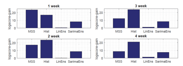
Moreover, as shown in Fig.3, the novel Gaussian process regression framework outperformed all benchmarks for four different targets [math]\displaystyle{ (T = 1,\ldots, 4) }[/math] , including LinEns, when compared using the official CDC scoring criterion log-score. Log-score describes the logarithmic probability of the forecast being within in an interval around the true value.


