Adversarial Fisher Vectors for Unsupervised Representation Learning: Difference between revisions
| Line 109: | Line 109: | ||
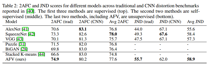
As AFVs transform data from feature space to the paramter space of the generative model and as a result carry information about data manifold, they are also expected to carry additional fine-grained perceptual information. To evaluate this, authors ran experiments to examine the usefulness of AFVs as a perceptual similarity metric consistent with human judgments. They use the AFV representation to calculate distances between image patches and compare with current methods on the Berkeley-Adobe Perceptual Patch Similarity (BAPPS) dataset on 2AFC and Just Noticeable Difference (JND) metrics. They trained a GAN on ImageNet and then calculate AFVs on the BAPPS evaluation set. | As AFVs transform data from feature space to the paramter space of the generative model and as a result carry information about data manifold, they are also expected to carry additional fine-grained perceptual information. To evaluate this, authors ran experiments to examine the usefulness of AFVs as a perceptual similarity metric consistent with human judgments. They use the AFV representation to calculate distances between image patches and compare with current methods on the Berkeley-Adobe Perceptual Patch Similarity (BAPPS) dataset on 2AFC and Just Noticeable Difference (JND) metrics. They trained a GAN on ImageNet and then calculate AFVs on the BAPPS evaluation set. | ||
Table 2 shows the performance of AFV along with a variety of existing benchmarks. Clearly, AFV exceeds the reported unsupervised and self-supervised methods and is competitive with supervised methods trained on ImageNet. | Table 2 shows the performance of AFV along with a variety of existing benchmarks. Clearly, AFV exceeds the reported unsupervised and self-supervised methods and is competitive with supervised methods trained on ImageNet. | ||
[[File:Sobhan_Table2.png]] | |||
Revision as of 11:14, 15 November 2020
Introduction
Generative adversarial networks (GANs) are one of the most important generative models, where a couple of discriminator and generator compete to each other to solve a minimax game. Based on the original GAN paper, when the training is finished and Nash Equilibrium is reached, the discriminator is nothing but a constant function that assigns a score of 0.5 everywhere. This means that in this setting discriminator is nothing more than a tool to train the generator. Furthermore, the generator in traditional GAN model the data density in an implicit manner while in some applications we need to have an explicit generative model of data. Recently, it has been shown that training an energy-based model (EBM) with a parameterized variational is also a similar minimax game similar to the one in GAN. Although they are similar, There is an advantage of this EBM view that is unlike the original GAN formulation, in this EBM model discriminator itself is an explicit density model of the data.
Considering some remarks, authors in this paper show that an energy-based model can be trained using similar minmax formulation in GANs. After training the energy based model, the use Fisher Score and Fisher Information (which are calculated based on derivative of the generative models w.r.t its parameters) to evaluate the power of discriminator in modelling data distribution. More precisely, they calculate normalized Fisher Vectors and Fisher Distance measure using the derivative of the discriminator to estimate similarities both between individual data samples and between sets of samples. They name these derived representations Adversarial Fisher Vectors (AFVs). In fact fisher vector is a powerful representation that can be calculated using EBMs thanks to the fact that with respect to its parameter thanks to the fact that in this EBM model discriminator itself is an explicit density model of the data. Fisher vector can be used for set representation problem which is a challenging taks. In fact, as we will see, we can use fisher kernel to calculate distance between two set of images which is not a trivial task. Authors use AFV useful as pre-trained features for the following tasks:
- State-of-the-art performance for unsupervised feature extraction and linear classification tasks
- They used the similarity function induced by the learned density model as a perceptual metric that correlates well with human judgments
- They improve training of the GAN through monitoring (AFV metrics) and stability (MCMC updates) which is a difficult task in general.
- They use AFV to estimate distance between sets which allow them monitor the training process. More precisely, They show that the Fisher Distance between the set of validation examples and generated examples can effectively capture the existence of overfitting.
Background
Generative Adversarial Networks
The weights of generator and discriminator are updated by solving the following optimization problem: \begin{equation} \underset{G}{\text{max}} \ \underset{D}{\text{min}} \ E_{\mathbf{x} \sim p_{data(\mathbf{x})}}[-\log D(\mathbf{x})]- E_{\mathbf{z} \sim p_{\mathbf{z}}(\mathbf{z})}[-\log (1-D(G(\mathbf{z})))] \tag{1} \label{1} \end{equation}
Where [math]\displaystyle{ p_{data(\mathbf{x})} }[/math], [math]\displaystyle{ D(x) }[/math], and [math]\displaystyle{ G(x) }[/math] are distribution of data, discriminator, and generator respectively. To optimize the above problem, in the inner loop [math]\displaystyle{ D }[/math] is trained until convergence given [math]\displaystyle{ G }[/math], and in the outer loop [math]\displaystyle{ G }[/math], is updated one step given [math]\displaystyle{ D }[/math].
GANs as variational training of deep EBMs
Assume an energy based model define a density function [math]\displaystyle{ p_{E}(\mathbf{x}) }[/math] as [math]\displaystyle{ \frac{e^{-E(\mathbf{x})}}{ \int_{\mathbf{x}} e^{-E(\mathbf{x})} \,d\mathbf{x} } }[/math]. Then, the negative log likelihood (NLL) of the [math]\displaystyle{ p_{E}(\mathbf{x}) }[/math] can be written as
\begin{equation} E_{\mathbf{x} \sim p_{data(\mathbf{x})}}[E(\mathbf{x})]+ \log \int_{\mathbf{x}} q(\mathbf{x}) \frac{e^{-E(\mathbf{x})}} {q(\mathbf{x})}\,d\mathbf{x} = E_{\mathbf{x} \sim p_{data(\mathbf{x})}}[E(\mathbf{x})]+ \log E_{\mathbf{x} \sim q(\mathbf{x})}[\frac{e^{-E(\mathbf{x})}} {q(\mathbf{x})}] \geq \\ E_{\mathbf{x} \sim p_{data(\mathbf{x})}}[E(\mathbf{x})]+ E_{\mathbf{x} \sim q(\mathbf{x})}[\log \frac{e^{-E(\mathbf{x})}} {q(\mathbf{x})}]= E_{\mathbf{x} \sim p_{data(\mathbf{x})}}[E(\mathbf{x})]- E_{\mathbf{x} \sim q(\mathbf{x})}[E(\mathbf{x})] + H(q) \tag{2} \label{2} \end{equation}
where [math]\displaystyle{ q(x) }[/math] is an auxiliary distribution which is called call the variational distribution and [math]\displaystyle{ H(q) }[/math] its entropy. Here Jensen’s inequality was used to obtain the variational lower bound on the NLL given [math]\displaystyle{ H(q) }[/math]. This bound is tight if [math]\displaystyle{ q(x) \propto e^{-E(\mathbf{x})} \ \forall \mathbf{x}, }[/math] which means [math]\displaystyle{ q(x) = p_{E}(\mathbf{x}) }[/math]. In this case, if we put [math]\displaystyle{ D(\mathbf{x})= -E(\mathbf{x}) }[/math] and also [math]\displaystyle{ q(x)= p_{G}(\mathbf{x}) }[/math] the Eq.\ref{2} turn to the following problem:
\begin{equation} \underset{D}{\text{min}} \ \underset{G}{\text{max}} \ E_{\mathbf{x} \sim p_{data(\mathbf{x})}}[-\log D(\mathbf{x})]+ E_{\mathbf{z} \sim p_{\mathbf{z}}(\mathbf{z})}[\log (D(G(\mathbf{z})))] +H(p_{G}) \tag{3} \label{3} \end{equation}
where in the problem, the variational lower bound is maximized w.r.t. [math]\displaystyle{ p_{G} }[/math]; the energy model then is updated one step to decrease the NLL with the optimal [math]\displaystyle{ p_{G} }[/math] (see Figure1). 
Equations \ref{3} and \ref{1} are similar in the sense that both taking the form of a minimax game between [math]\displaystyle{ D }[/math] and [math]\displaystyle{ G }[/math]. However, there are 3 major differences:
- The entropy regularization term [math]\displaystyle{ H(p_{G}) }[/math] in Eq. \ref{3} prevents the generator from collapsing (although in practice, it is difficult to come up with a differentiable approximation to the entropy term [math]\displaystyle{ H(p_{G}) }[/math] and instead heuristic regularization methods such as Batch Normalization are used).
- the order of optimizing [math]\displaystyle{ D }[/math] and [math]\displaystyle{ G }[/math] is different.
- More importantly, [math]\displaystyle{ D }[/math] is a density model for the data distribution and [math]\displaystyle{ G }[/math] learns to sample from [math]\displaystyle{ D }[/math].
Methodology
Adversarial Fisher Vectors
As it was mentioned, one the most important advantageous of an EBM GAN compared with traditional ones is that the discriminator is a dual form of the generator. This means that the discriminator can define a distribution that matches the training data. Generally, there is a straightforward way for evaluating the quality of generator and that is inspecting the quality of produced samples. However, when it comes to discriminator, this is not clear how to evaluate or use a discriminator rained in minmax scheme. To evaluate and also employ discriminator of the GAN, authors in this paper propose to employ the theory of Fisher Information. This theory was proposed by motivation of making connection between two different types of models used in machine learning i.e, generative and discriminator models. Given a density model [math]\displaystyle{ p_{\theta}(\mathbf{x}) }[/math] where [math]\displaystyle{ \mathbf{x} \in R^d }[/math] and [math]\displaystyle{ \theta }[/math] are input and model parameters, the fisher score of an example [math]\displaystyle{ \mathbf{x} }[/math] is defined as [math]\displaystyle{ U_\mathbf{x}=\nabla_{\theta} \log p_{\theta}(\mathbf{x}) }[/math]. This gradient maps an example [math]\displaystyle{ \mathbf{x} }[/math] into a feature vector that is a point in the gradient space of the manifold. Intuitively, This gradient [math]\displaystyle{ U_\mathbf{x} }[/math] can be used to define the direction of steepest ascent in [math]\displaystyle{ \log p(\mathbf{x}|\theta) }[/math] for the example [math]\displaystyle{ \mathbf{x} }[/math] along the manifold. In other words, The Fisher Score encodes the desired change of model parameters to better fit the example [math]\displaystyle{ \mathbf{x} }[/math]. The authors define the Fisher Information as [math]\displaystyle{ I=E_{\mathbf{x} \sim} p_{\theta}(\mathbf{x}) [U_\mathbf{x} U_\mathbf{x}^T] }[/math]. Having Fisher Information and Fisher Score, one can then map an example [math]\displaystyle{ \mathbf{x} }[/math] from feature space to the model space, and measure the proximity between two examples [math]\displaystyle{ \mathbf{x} }[/math]; [math]\displaystyle{ \mathbf{y} }[/math] by [math]\displaystyle{ U_\mathbf{x}^T I^{-1} U_\mathbf{y} }[/math]. The metric distance based on this proximity is defined as [math]\displaystyle{ (U_\mathbf{x}-U_\mathbf{y})^T I^{-1} (U_\mathbf{x}-U_\mathbf{y}) }[/math]. This metric distance is called Fisher distance and easily can be generalized to measure distance between two sets. Finally, The adversarial Fisher Distance (AFV) is defined as
\begin{equation}
V_\mathbf{x}=I^{-\frac{1}{2}}U_\mathbf{x}
\end{equation}
As aresult, Fisher Distance is equivalent to the Euclidean distance with AFVs. The fisher vector theory has been use using simple generative models like gmms. In the domain of the EBMs, where the density model is parameterized as [math]\displaystyle{ p_\theta(\mathbf{x})= \frac{e^{-D(\mathbf{x},\theta)}}{\int_{\mathbf{x}} e^{-D(\mathbf{x},\theta)} \,d\mathbf{x}} }[/math] and [math]\displaystyle{ \theta }[/math] are parameters of [math]\displaystyle{ D }[/math], the fisher score is derived as
\begin{equation}
U_\mathbf{x}=\nabla_{\theta} D(\mathbf{x};\theta) - \nabla_{\theta} \log \int_{\mathbf{x}} e^{D(\mathbf{x},\theta)} \,d\mathbf{x}= \nabla_{\theta} D(\mathbf{x};\theta) - E_{\mathbf{x} \sim p_\theta(\mathbf{x})} \nabla_{\theta} D(\mathbf{x};\theta).
\tag{4}
\label{4}
\end{equation}
As we know, in an EBM GAN, the generator is updated during the training to match the distribution of [math]\displaystyle{ p_G(\mathbf{x}) }[/math] to [math]\displaystyle{ p_\theta(\mathbf{x}) }[/math]. This allows us to approximate the second term in Eq.\ref{4} by sampling form generator's distribution which let us to compute the Fisher Information and Fisher Score in EBM GAN as follow:
\begin{equation} U_\mathbf{x}=\nabla_{\theta} D(\mathbf{x};\theta) - E_{\mathbf{z} \sim p(\mathbf{z})} \nabla_{\theta} D(G(\mathbf{z});\theta), \quad I= E_{\mathbf{z} \sim p(\mathbf{z})}[U_{G(\mathbf{z})} U^T_{G(\mathbf{z})}] \tag{5} \label{5} \end{equation}
Finally, having Fisher Score and Fisher Information, we use the following approximation to calculate AFV:
\begin{equation}
V_\mathbf{x}=\mbox{diag}(I)^{-\frac{1}{2}}U_\mathbf{x}
\tag{6}
\label{6}
\end{equation}
Remember that by using Fisher Score, we transform data from feature space to the parameter space which means that the dimensionality of the vectors can be vectors can easily be up to millions. As a result, replacing [math]\displaystyle{ I }[/math] with [math]\displaystyle{ \mbox{diag}(I) }[/math] is an attempt to reduce the computational load of calculating final AFV.
Experiments
Evaluating AFV representations
As it was pointed out, the main advantage of the EBM GANs is their powerful discriminator which is able to learn a density function that characterizes the data manifold of the training data. To evaluate how good the discriminator learns the data distribution, authors proposed to use Fisher Information theory. To do this, authors trained some models under different models and employed the discriminator to extract AFVs and then use these vectors for unsupervised pretraining classification task. Results in Table 1 suggest that AFVs achieve state-of-art performance in unsupervised pretraining classification task and also comparable with the supervised learning.
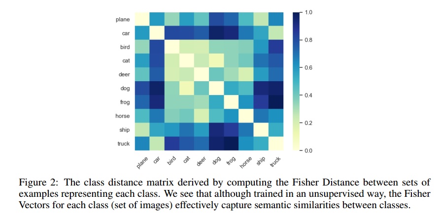
AFVs can also be used to measure distance between a set of data points. Authors took advantage of this point and calculate the semantic distance between classes (all data points of every class) in CIFAR 10. As can be seen from Figure 2, although the training has been unsupervised, the semanit relation between classed are well estimated. For example, in Figure 2 cars are similar to trucks, dogs are similar to cats.
An interesting point about AFVs is theie robustness to overfitting. AFVs are 3 orders of magnitude higher than those of the existing methods, which would typically bring a higher propensity to overfitting. However, AFVs still show great generalization ability, demonstrating that they are indeed encoding a meaningful low dimensional subspace of original data.
As AFVs transform data from feature space to the paramter space of the generative model and as a result carry information about data manifold, they are also expected to carry additional fine-grained perceptual information. To evaluate this, authors ran experiments to examine the usefulness of AFVs as a perceptual similarity metric consistent with human judgments. They use the AFV representation to calculate distances between image patches and compare with current methods on the Berkeley-Adobe Perceptual Patch Similarity (BAPPS) dataset on 2AFC and Just Noticeable Difference (JND) metrics. They trained a GAN on ImageNet and then calculate AFVs on the BAPPS evaluation set. Table 2 shows the performance of AFV along with a variety of existing benchmarks. Clearly, AFV exceeds the reported unsupervised and self-supervised methods and is competitive with supervised methods trained on ImageNet.


