Physics-informed neural networks: A deep learning framework for solving forward and inverse problems involving nonlinear partial differential equations

Presented by

Cameron Meaney

Introduction

In recent years, there has been an enormous growth in the amount of data and computing power available to researchers. Unfortunately, for many real-world scenarios, the cost of data acquisition is simply too high to collect an amount of data sufficient to guarantee robustness or convergence of training algorithms. In such situations, researchers are faced with the challenge of trying to generate results based on partial or incomplete datasets. Regularization techniques or methods which can artificially inflate the dataset become particularly useful in these situations; however, such techniques are often highly dependent of the specifics of the problem.

Luckily, in important real-world scenarios that we endeavor to analyze, there is often a wealth of existing information from which we can draw. This existing information commonly manifests in the form of a mathematical model, particularly a set of partial differential equations (PDEs). In this paper, the authors provide a technique for incorporating the information of a physical system contained in a PDE into the optimization of a deep neural network. This technique is most useful in situations where established PDE models exist, but where our amount of available data is too small to guarantee robustness or convergence in neural network training. In essence, the accompanying PDE model can be used as a regularization agent, constraining the space of acceptable solutions to help the optimization converge more quickly and more accurately.

Problem Setup

Consider the following general PDE,

\begin{align*} u_t + N[u;\vec{\lambda}] = 0, \end{align*}

where [math]\displaystyle{ u }[/math] is the function we wish to find, subscripts denote partial derivatives, [math]\displaystyle{ \vec{\lambda} }[/math] is the set of parameters on which the PDE depends, and [math]\displaystyle{ N }[/math] is a differential, potentially nonlinear operator. This general form encompasses a wide array of PDEs used across the physical sciences including conservation laws, diffusion processes, advection-diffusion-reaction systems, and kinetic equations. Suppose that we have noisy measurements of the PDE solution, [math]\displaystyle{ u }[/math], scattered across the spatio-temporal input domain. Then, we are interested in answering two questions about the physical system:

(1) Given fixed model parameters, [math]\displaystyle{ \vec{\lambda} }[/math], what can be said about the unknown hidden state [math]\displaystyle{ u(t,x) }[/math]?

and

(2) What set of parameters, [math]\displaystyle{ \vec{\lambda} }[/math], best describe the observed data for this PDE system?

Data-Driven Solutions of PDEs

We will begin by attempting to answer the first of the questions above. Specifically, if given a small amount of noisy measurements of the solution of the PDE

\begin{align*} u_t + N[u] = 0, \end{align*}

can we estimate the full solution, [math]\displaystyle{ u(t,x) }[/math], by approximating it with a deep neural network? Note that [math]\displaystyle{ \vec{\lambda} }[/math] no longer appears in the operator because we assume those values to be known. Approximating the solution of the PDE with a neural network results in what the authors refer to as a 'Physics-Informed Neural Network' (PINN). Importantly, this technique is most useful when we are in the small-data regime - for if we had lots of data, it simply wouldn't be necessary to include information from the PDE because the data alone would be sufficient. In these examples, we are seeking to learn from a very small amount of data which makes information from the PDE necessary to include in order to generate meaningful results.

The paper details two cases of data: continuous-time and discrete-time. Both cases are detailed individually below.

Continuous-Time Models

Consider the case where our noisy measurements of the solution are randomly scattered across the spatio-temporal input domain. This case is referred to as the continuous-time case. We define the function

\begin{align*} f = u_t + N[u] \end{align*}

as the left hand side of the PDE above. Now assume that the PDE solution, [math]\displaystyle{ u(t,x) }[/math], can be approximated by a deep neural network. Therefore, the function [math]\displaystyle{ f(t,x) }[/math] can also be approximated by a neural network since it is simply a function of [math]\displaystyle{ u(t,x) }[/math]. In order to calculate [math]\displaystyle{ f(t,x) }[/math] as a function of [math]\displaystyle{ u(t,x) }[/math], derivates of the network [math]\displaystyle{ u(t,x) }[/math] will need to be taken with respect to its inputs. This network differentiation is accomplished using a technique called automatic differentiation [2]. Importantly, the weights of the two neural networks will be shared, since [math]\displaystyle{ f(t,x) }[/math] is simply a function of [math]\displaystyle{ u(t,x) }[/math]. The key idea in finding this shared set of weights is to train the networks with a loss function that has two distinct parts. The first part quantifies how well the neural network satisfies the known data points and is given by:

\begin{align*} MSE_u = \frac{1}{N_u} \sum_{i=1}^{N_u} [u(t_u^i,x_u^i) - u^i]^2 \end{align*}

where the summation is over the set of known data points. The second part of the loss function quantifies how well the neural network satisfies the PDE and is given by:

\begin{align*} MSE_f = \frac{1}{N_u} \sum_{i=1}^{N_u} [f(t_u^i,x_u^i)]^2. \end{align*}

Notice that since [math]\displaystyle{ f }[/math] is all of the PDE terms moved to one side of the equation, the closer that [math]\displaystyle{ f }[/math] is to zero, the better that the neural network satisfies to PDE. The full loss function used in the optimization is then taken to be the sum of these two parts:

\begin{align*} MSE = MSE_u + MSE_f. \end{align*}

By using this loss function in the optimization, information from both the known data and the known physics (from PDE) can be incorporated into the neural network. This effectively regularizes the optimization, allowing for the network to learn from a smaller number of datapoints than would otherwise be necessary. An example of this method can be seen in figure 1.

Discrete-Time Models

Now consider the case where our available data is not randomly scattered across the spatio-temporal domain, but rather only present at two particular times. This is known as the discrete-time case and occurs frequently in real-world examples such as when dealing with discrete pictures or medical images with no data between them. These cases and can be dealt with in the same manner as the continuous case with a few small adjustments. To adapt the PINN technique to discrete time models, we must leverage Runge-Kutta methods for numerical solutions of differential equations [?]. Runge-Kutta methods approximate the solution of a differential equation at the next numerical time step by first approximating the solution at a set of intermediate points between the time steps, then using these values to predict the full time step. The general form of a Runge-Kutta method with [math]\displaystyle{ q }[/math] stages is given by:

\begin{align*} u^{n+c_i} &= u^n - \Delta t \sum^q_{j=1} a_{ij} N[u^{n+c_j}], ~ i = 1,...,q \\ u^{n+1} &= u^n - \Delta t \sum^q_{j=1} b_j N[u^{n+c_j}] \end{align*}

where [math]\displaystyle{ u^{n+c_j} = u(t^n + c_j \Delta t, x) }[/math] and the general form includes both explicit and implicit time-stepping schemes. For more information of Runge-Kutta methods, see [?].

In the continuous-time case, we had approximated the function [math]\displaystyle{ u(t,x) }[/math] by a neural network. Therefore, our neural network approximation for [math]\displaystyle{ u(t,x) }[/math] had two inputs and one output. In the discrete case, instead of creating a neural netowrk which takes [math]\displaystyle{ t }[/math] and [math]\displaystyle{ x }[/math] as input and outputs the value of [math]\displaystyle{ u(t,x) }[/math], we create a neural network which only takes [math]\displaystyle{ x }[/math] and outputs the values of the solution at the intermediate points of the Runge-Kutta time-stepping scheme, [math]\displaystyle{ [u^{n+c_j}] }[/math] for [math]\displaystyle{ i=1,...,q }[/math]. Therefore, the PINN that we create here has one input and [math]\displaystyle{ q }[/math] outputs. Importantly, information from the PDE is now incorporated into the the Runge-Kutta time-stepping scheme, so we do not need to add a term to the loss function to include it. Instead, our discrete-time loss function consists of two parts - one to quantify agreement with the data at the time of the initial data snapshot and one to quantify the agreement with data at the final data snapshot. For an example of this, see figure ?.

Data-Driven Discovery of PDEs

After having answered the first question, we can turn our focus to the second question. Specifically, if given a small amount of noisy measurements of the solution of the PDE

\begin{align*} u_t + N[u;\vec{\lambda}] = 0, \end{align*}

can we estimate the values of the parameters, [math]\displaystyle{ \vec{\lambda} }[/math], that best describe the observed data? The difference between this case and the above is that we no longer know the values of the parameters [math]\displaystyle{ \vec{\lambda} }[/math] appearing in the PDE. The procedure is, in essence, unchanged other than we now treat the PDE parameters as trainable parameters of the neural network. Since the discovery case outlined here is an extension of the solution case outlined above, the examples given below include unknown parameters and should therefore cover the full procedure.

Examples

While the paper gives many examples of the PINN method, three are outlined here to demonstrate the method's utility.

Continuous-Time Example

For an example of this method in action, consider a problem involving Burger's equation, given by:

\begin{align*} &u_t + uu_x - (0.01/\pi)u_{xx} = 0, ~ x \in [-1,1], ~ t \in [0,1], \\ &u(0,x) = -\sin(\pi x), \\ &u(t, -1) = u(t,1) = 0. \end{align*}

Notably, Burger's equation is known as a challenging problem to solve because of the shock (discontinuity) that forms after sufficiently large time. However, using PINNs, this shockwave is easily handled.

So, assume that we are given noisy measurements of the solution of Burger's equation scattered across the spatio-temporal domain. Also assume that we do not know the values of the parameters in Burger's equation - we only know the equation form:

\begin{align*} &u_t + \lambda_1 uu_x - \lambda_2 u_{xx} = 0. \end{align*}

Additionally, we also assume that we are ignorant of the initial conditions and boundary conditions which generate the solution. Importantly, information form the initial and boundary conditions is contained in the known data points. We define the function [math]\displaystyle{ f(t,x) }[/math] as:

\begin{align*} f = u_t + \lambda_1 uu_x - \lambda_2 u_{xx} \end{align*}

and assume that [math]\displaystyle{ u(t,x) }[/math] is approximated by a deep neural network - hence creating a PINN. Then, the shared parameters of the neural networks for [math]\displaystyle{ u(t,x) }[/math] and [math]\displaystyle{ f(t,x) }[/math] as well as the parameters [math]\displaystyle{ \lambda_1 }[/math] and [math]\displaystyle{ \lambda_2 }[/math] are simultaneously learned by minimizing the combined loss function [math]\displaystyle{ MSE = MSE_u + MSE_f }[/math] as defined above.

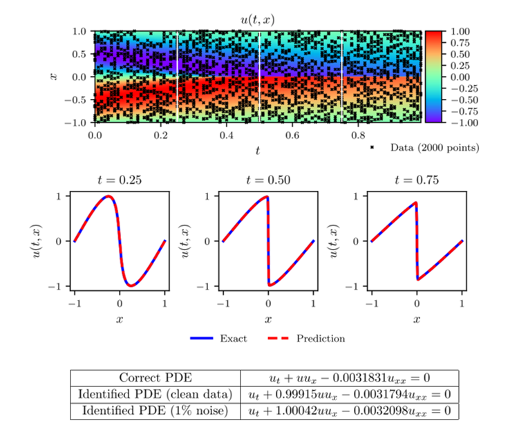
For this example, assume that we have 2000 datapoints across the entire spatio-temporal domain (representing a mere 2.0% of the known data). The correct values of the parameters which are used to generate the datapoints are [math]\displaystyle{ \lambda_1 = 1.0 }[/math] and [math]\displaystyle{ \lambda_2 = 0.01/\pi }[/math]. Also assume that the value of the solution for each of the known datapoints is randomly perturbed by up to 1% of its value - making the dataset noisy. This problem is trained using the procedure outlined above with a deep neural network of 9 layers with 20 neurons per hidden layer and using the L-BFGS optimizer.

The results of this example can be seen in figure 1. In the top panel, the exact solution can be seen with the datapoints selected for training pointed out. In the middle panel, a comparison of the exact and predicted solutions can be seen for three different times showing the accuracy of the PINN prediction. In the bottom panel, a comparison of the exact and predicted parameter values can also be seen. Also included in this bottom panel is the parameter predictions for the noiseless data case for comparison. Notice the remarkable accuracy with which the PINN is able to predict the correct parameter values in both noisy and noiseless cases. In figure 2, a comparison of the error in the predicted parameter values for different amounts of known data and noise.

Figure 1

Figure 2

Discrete-Time Example

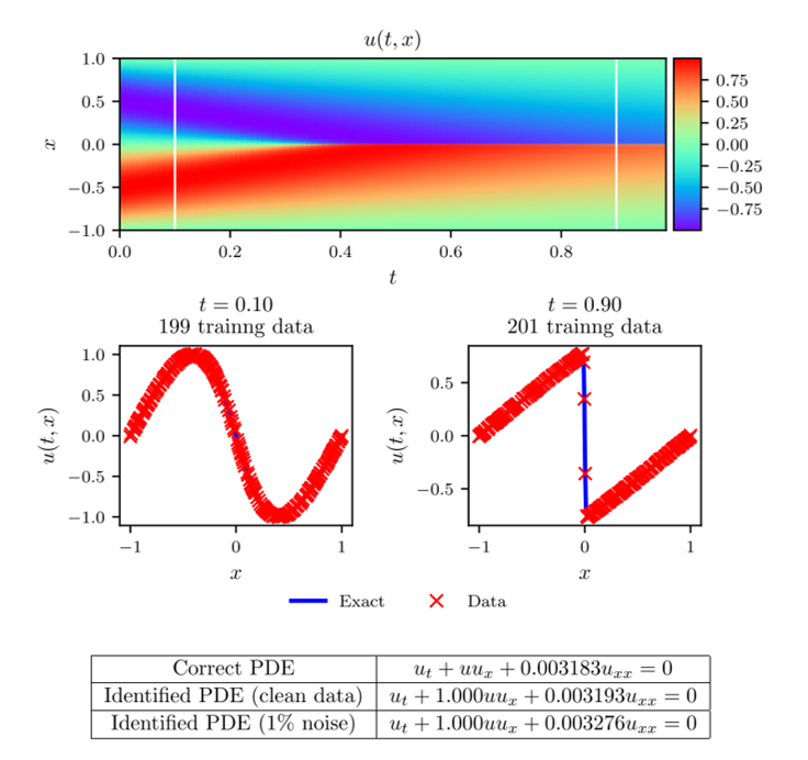
For a discrete-time example, let us again consider the Burger's equation but only allow ourselves data at two time snapshots. Specifically, our known data consists of 199 points at time [math]\displaystyle{ t=0.1 }[/math] and 201 points at [math]\displaystyle{ t=0.9 }[/math]. The correct parameter values and dataset noise is the same as in the continuous case and the procedure is as explained in the discrete-time section above. The neural network consists of four layers with 50 neurons per hidden layer. We choose the number of Runge-Kutta stages to be [math]\displaystyle{ q=500 }[/math], meaning that we approximate the solution at 500 intermediate time points. Note that the theoretical error estimates for a Runge-Kutta scheme with 500 stages is far below machine precision (truncation error of [math]\displaystyle{ O(\Delta t^{2q}) }[/math]).

The results of this example can be seen in figure 3. In the figure, the top panel shows the exact solution of Burger's equation with the known data at [math]\displaystyle{ t=0.1 }[/math] and [math]\displaystyle{ t=0.9 }[/math]. In the middle panel, the exact solution and predicted solution are compared at the two time snapshots. In the bottom panel, the predicted parameter values are reported for noisy and noiseless data. Notice the accuracy with which the network can predict the parameter values.

Figure 3

Navier-Stokes with Pressure

Naturally, there are many extensions to the base problem that the PINN method tackles. One particularly interesting example of this is illustrated in the following example.

Consider the Navier-Stokes equations in two dimensions, given by:

\begin{align*} u_t + \lambda_1 ( uu_x + vu_y) = -p_x + \lambda_2 (u_xx + u_yy) \\ v_t + \lambda_1 (uv_x + vv_y) = -p_y + \lambda_2 (v_xx + v_yy) \end{align*}

where [math]\displaystyle{ u }[/math] and [math]\displaystyle{ v }[/math] are the [math]\displaystyle{ x }[/math] and [math]\displaystyle{ y }[/math] components of the fluid velocity. In these equations, not only are there two unknown parameters, [math]\displaystyle{ \lambda_1 }[/math] and [math]\displaystyle{ \lambda_2 }[/math], but there is also an entire unknown pressure field, [math]\displaystyle{ p(t,x,y) }[/math]. Based on the physics of the problem, we can assume that there is a scalar function [math]\displaystyle{ \psi }[/math] which satisfies [math]\displaystyle{ \psi_y = u }[/math] and [math]\displaystyle{ \psi_x = -v }[/math]. Assume that we have noisy measurements of the velocity field scattered across the spatio-temporal domain.

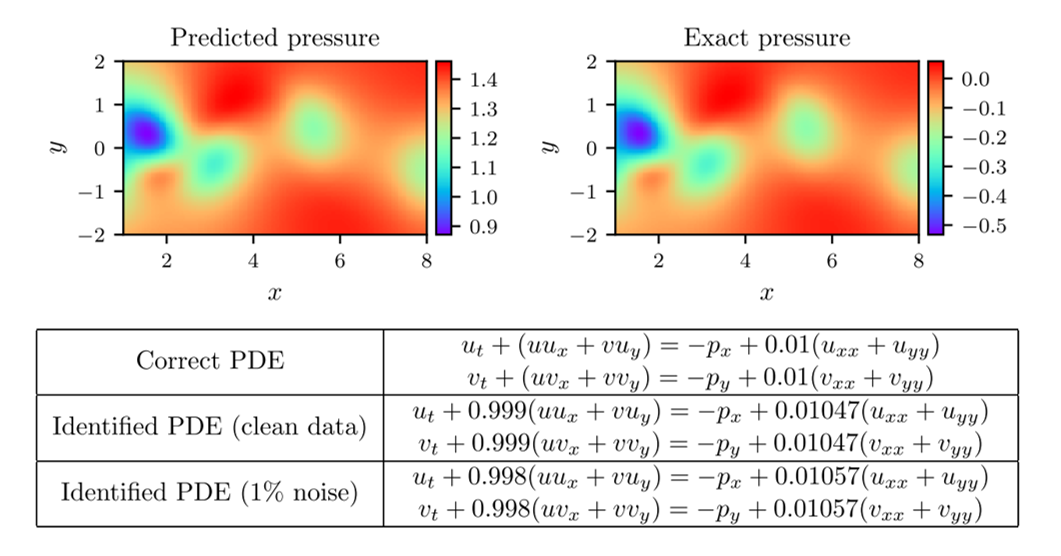
We approximate [math]\displaystyle{ \psi }[/math] with a PINN, proceeding as we did in the continuous case above with the addition of also approximating the pressure field with a neural network. With each training batch, the weights of both networks are updated. We can compute the components of the velocity by differentiating the network for [math]\displaystyle{ \psi }[/math]. Our full loss function is defined as in the continuous case, but note that the term quantifying the satisfaction of the PDEs will depend on the pressure network.

We allow ourselves 1% of the total data and optimize the network as we did before. The network has 9 layers with 20 neurons per hidden layer. See the results of this in figure ?.

Conclusion

This paper introduces physics-informed neural networks, a novel type of function-approximator neural network that utilize existing information of physical systems in order to train using a small amount of data. It does this by incorporating information from a governing PDE model into the loss function. It allows for prediction of the full solution, incorporation of noise into the measurements, estimation of model parameters appearing in the PDE, and approximation of auxiliary functions appearing in the PDE. A variation of the main technique allows for predictions originating from discrete-time data.

PINNs are a powerful technique with many possible extensions. This paper and related papers by this group have received many citations and they are actually patenting this technique.

References

[1] Raissi, M., Perdikaris, P., & Karniadakis, G. E. (2019). Physics-informed neural networks: A deep learning framework for solving forward and inverse problems involving nonlinear partial differential equations. Journal of Computational Physics, 378, 686–707.

[2] A. G. Baydin, B. A. Pearlmutter, A. A. Radul, J. M. Siskind, Au- tomatic differentiation in machine learning: a survey, arXiv preprint arXiv:1502.05767 (2015).