User:Bsharman: Difference between revisions
No edit summary |
No edit summary |
||
| Line 68: | Line 68: | ||
1.Multiple Linear Regression: In MLR, the relationship between the dependent and the two or more independent variables is predicted by fitting a linear model. The model parameters are calculated by minimizing the sum of squares of the errors. The significance of the variables is determined by tests like the F test and the p-values. | 1.Multiple Linear Regression: In MLR, the relationship between the dependent and the two or more independent variables is predicted by fitting a linear model. The model parameters are calculated by minimizing the sum of squares of the errors. The significance of the variables is determined by tests like the F test and the p-values. | ||
2. | 2.REPTree: REPTree stands for reduced error pruning tree. It can build both classification and regression trees, depending on the type of the response variable. In this case, it uses regression tree logic and creates many trees across several iterations. This algorithm develops these trees based on the principles of information gain and variance reduction. At the time of pruning the tree, the algorithm uses the lowest mean square error to select the best tree. | ||
3.Random Tree: A random tree selects some of the attributes at each node in the decision tree and builds a tree based on random selection of data as well as attributes. Random Tree does not do pruning. Instead, it estimates class probabilities based on a hold-out set. | 3.Random Tree (Also known as the Random Forest): A random tree selects some of the attributes at each node in the decision tree and builds a tree based on random selection of data as well as attributes. Random Tree does not do pruning. Instead, it estimates class probabilities based on a hold-out set. | ||
4.Artificial Neural Network: In a neural network, the inputs are transformed into outputs via a series of layered units where each of these units transforms the input received by it via a function into an output that gets further transmitted to units down the line. The weights that are used to weigh the inputs are improved after each iteration via a method called backpropagation in which errors propagate backward in the network and are used to update the weights to make the computed output closer to the actual output. | 4.Artificial Neural Network: In a neural network, the inputs are transformed into outputs via a series of layered units where each of these units transforms the input received by it via a function into an output that gets further transmitted to units down the line. The weights that are used to weigh the inputs are improved after each iteration via a method called backpropagation in which errors propagate backward in the network and are used to update the weights to make the computed output closer to the actual output. | ||
| Line 117: | Line 117: | ||
Using the PCA method, Multiple Linear Regression showed the best results with MAE and RMSE values of 1.64 and 2.06 respectively. With CFS, REPTree had the highest accuracy with MAE and RMSE values of 1.52 and 2.02 respectively. | Using the PCA method, Multiple Linear Regression showed the best results with MAE and RMSE values of 1.64 and 2.06 respectively. With CFS, REPTree had the highest accuracy with MAE and RMSE values of 1.52 and 2.02 respectively. | ||
Further work can be directed towards dealing all the variables rather than deleting the ones where more than 30% of the values are missing. Customer segmentation, i.e. grouping customers based on their profiles can help companies come up with customized policy for each group. This can be done via unsupervised algorithms like clustering. Work can also be done to make the models more explainable especially if we are using PCA and ANNs to analyze data. We can also get indirect data about the prospective applicant like their driving behavior, education record etc to see if these attributes contribute to better risk profiling than the already available data. | Further work can be directed towards dealing all the variables rather than deleting the ones where more than 30% of the values are missing. Customer segmentation, i.e. grouping customers based on their profiles can help companies come up with customized policy for each group. This can be done via unsupervised algorithms like clustering. Work can also be done to make the models more explainable especially if we are using PCA and ANNs to analyze data. We can also get indirect data about the prospective applicant like their driving behavior, education record etc to see if these attributes contribute to better risk profiling than the already available data. | ||
'''Critics''' | |||
---- | |||
Since the project built multiple models and had utilized various methods to evaluate the result. They could potentially ensemble the prediction, such as averaging the result of the different models, to achieve a better accuracy result. Another method is model stacking, we can input the result of one model as input into another model for better results. However, they do have some major setbacks: sometimes, the result could be effect negatively (ie: increase the RMSE). In addition, if the improvement is not prominent, it would make the process much more complex thus cost time and effort. In a research setting, stacking and ensembling are definitely worth a try. In a real-life business case, it is more of a trade-off between accuracy and effort/cost. | |||
'''References''' | '''References''' | ||
Revision as of 16:06, 6 October 2020
Risk prediction in life insurance industry using supervised learning algorithms
Presented By
Bharat Sharman, Dylan Li, Leonie Lu, Mingdao Li
Introduction
Risk assessment lies at the core of the Life Insurance Industry. It is extremely important for a Life Insurance Company to assess the risk of an application accurately in order to make sure that applications with an actual low risk are accepted and an actual high risk are rejected. Otherwise, individuals with an unacceptably high risk profile will be issued policies and when they pass away, the company will face large losses due to high insurance payouts. Such a situation is called ‘Adverse Selection’, where individuals who are most likely to suffer losses take insurance and those who are not likely to suffer losses do not and thus, the company suffers losses as a result.
Traditionally, the process of Underwriting (deciding whether or not to insure the life of an individual) has been done using Actuarial calculations. Actuaries group customers according to their estimated levels of risk determined from historical data. (Cummins J, 2013) However, these conventional techniques are time consuming and it is not uncommon to take a month to issue a policy. They are expensive as a lot of manual processes need to be executed.
Predictive Analysis has emerged as a useful technique to streamline the underwriting process to reduce the time of Policy issuance and to improve the accuracy of risk prediction. In this paper, the authors use data from Prudential Life Insurance company and investigate the most appropriate data extraction method and the most appropriate algorithm to assess risk.
Literature Review
Before a Life Insurance company issues a policy, it must execute a series of underwriting related tasks. (Mishr, 2016)These tasks involve gathering extensive information about the applicant. The insurer has to analyze the employment, medical, family and insurance histories of the applicant and factor all of them into a complicated series of calculations to determine the risk rating of the applicant. On basis of this risk rating, premiums are calculated. (Prince, 2016)
In a competitive marketplace, customers need policies to be issued quickly and long wait times can lead to them switch to other providers. (Chen, 2016). In addition, the costs of doing the data gathering and analysis can be expensive. The insurance company bears the expenses of the medical examinations and if a policy lapses, then the insurer has to bear the losses of all these costs. (J Carson, 2017). If the underwriting process uses Predictive Analytics, then the costs and time associated with many of these processes can be reduced via streamlining.
Methods and Techniques
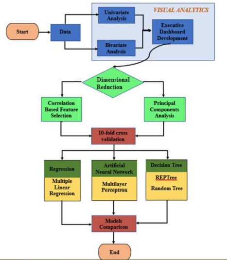
In Figure 1, the process flow of the analytics approach has been depicted. These stages will now be described in the following sections.
Description of the Dataset
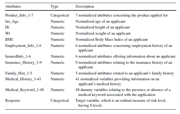
The data is obtained from the Kaggle competition hosted by the Prudential Life Insurance company. It has 59381 applications with 128 attributes. The attributes are continuous and discrete as well as categorical variables.
The data attributes, their types and the description is shown in Table 1 below:
Data Pre-Processing
In the data preprocessing step, missing values in the data are either imputed or those entries are dropped and some of the attributes are either transformed in a different form to make the subsequent processing of data easier.
Dimensionality Reduction
In this paper, there are two methods that have been used for dimensionality reduction –
1.Correlation based Feature Selection (CFS): This is a feature selection method in which a subset of features from the original features is selected. In this method, the algorithm selects features from the dataset that are highly correlated with the output but are not correlated with each other. The user does not need to specify the number of features to be selected. The correlation values are calculated based measures such a Pearson’s coefficient, minimum description length, symmetrical uncertainty and relief.
2.Principal Components Analysis (PCA): PCA is a feature extraction method that transforms existing features into new sets of features such that the correlation between them is zero and these transformed features explain the maximum variability in the data.
Supervised Learning Algorithms
The four Algorithms that have been used in this paper are the following:
1.Multiple Linear Regression: In MLR, the relationship between the dependent and the two or more independent variables is predicted by fitting a linear model. The model parameters are calculated by minimizing the sum of squares of the errors. The significance of the variables is determined by tests like the F test and the p-values.
2.REPTree: REPTree stands for reduced error pruning tree. It can build both classification and regression trees, depending on the type of the response variable. In this case, it uses regression tree logic and creates many trees across several iterations. This algorithm develops these trees based on the principles of information gain and variance reduction. At the time of pruning the tree, the algorithm uses the lowest mean square error to select the best tree.
3.Random Tree (Also known as the Random Forest): A random tree selects some of the attributes at each node in the decision tree and builds a tree based on random selection of data as well as attributes. Random Tree does not do pruning. Instead, it estimates class probabilities based on a hold-out set.
4.Artificial Neural Network: In a neural network, the inputs are transformed into outputs via a series of layered units where each of these units transforms the input received by it via a function into an output that gets further transmitted to units down the line. The weights that are used to weigh the inputs are improved after each iteration via a method called backpropagation in which errors propagate backward in the network and are used to update the weights to make the computed output closer to the actual output.
Experiments and Results
Missing Data Mechanism
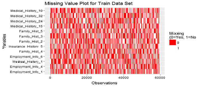
Attributes where more than 30% of Data was missing were dropped from Analysis. The data was tested for Missing Completely at Random (MCAR), one form of the nature of missing values using the Little Test. The null Hypothesis that the missing data was completely random had a p value of 0 meaning, MCAR was rejected. Then, all the variables were plotted to check how many missing values that they had and the results are shown in the figure below:
The variables that have the most number of missing variables are plotted at the top and that have the least number of missing variables are plotted at the bottom of the y-axis in the figure above. There does not seem to a pattern to the missing variables and therefore they are assumed to be Missing at Random (MAR).
Missing Data Imputation
Assuming that missing data follows an MAR pattern, multiple imputation is used as a technique to fill in the values of missing data. The steps involved in Multiple Imputation are the following:
Imputation: Imputation of the missing values is done over several steps and this results in a number of complete data sets. Imputation is done via a predictive model like linear regression to predict these missing values based on other variables in the data set.
Analysis: The complete data sets that are formed are analyzed and parameter estimates and standard errors are calculated.
Pooling: The analysis results are then integrated to form a final data set that is then used for further analysis.
Comparison of Feature Selection and Feature Extraction
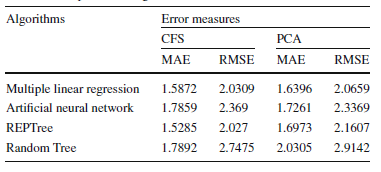
The Correlation based Feature Selection (CFS) method was performed using the Waikato Environment for Knowledge Analysis. It was implemented using a BestFirst search method on a CfsSubsetEval attribute evaluator. 33 variables were selected out the total of 117 features. PCA was implemented via a RankerSearch Method using a Principal Components Attributes Evaluator. Out of the 117 features, those that had a standard deviation of more than 0.5 times the standard deviation of the first principal component were selected and this resulted in 20 features for further analysis. After dimensionality reduction, this reduced data set was exported and used for building prediction models using the four machine learning algorithms discussed before – REPTree, Multiple Linear Regression, Random Tree and ANNs. The results are shown in the Table below:
For CFS, the REPTree model had the lowest MAE and RMSE. For PCA, Multiple Linear Regression Model had the lowest MAE as well as RMSE. So, for this dataset, it seems that overall, Multiple Linear Regression and REPTree Models are the two best ones in terms of lowest error rates. In terms of dimensionality reduction, it seems that CFS is a better method than PCA for this data set as the MAE and RMSE values are lower for all ML methods except ANNs.
Conclusion and Further Work
Predictive Analytics in the Life Insurance Industry is enabling faster customer service and lower costs by helping automate the process of Underwriting.
In this study, the authors analyzed data obtained from Prudential Life Insurance to predict risk scores via Supervised Machine Learning Algorithms. The data was first pre-processed to first replace the missing values. Attributes having more than 30% of missing data were eliminated from analysis.
Two methods of dimensionality reduction – CFS and PCA were used and the number of attributes used for further analysis were reduced to 33 and 20 via these two methods. The Machine Learning Algorithms that were implemented were – REPTree, Random Tree, Multiple Linear Regression and Artificial Neural Networks. Model validation was performed via a ten-fold cross validation. The performance of the models was evaluated using MAE and RMSE measures.
Using the PCA method, Multiple Linear Regression showed the best results with MAE and RMSE values of 1.64 and 2.06 respectively. With CFS, REPTree had the highest accuracy with MAE and RMSE values of 1.52 and 2.02 respectively.
Further work can be directed towards dealing all the variables rather than deleting the ones where more than 30% of the values are missing. Customer segmentation, i.e. grouping customers based on their profiles can help companies come up with customized policy for each group. This can be done via unsupervised algorithms like clustering. Work can also be done to make the models more explainable especially if we are using PCA and ANNs to analyze data. We can also get indirect data about the prospective applicant like their driving behavior, education record etc to see if these attributes contribute to better risk profiling than the already available data.
Critics
Since the project built multiple models and had utilized various methods to evaluate the result. They could potentially ensemble the prediction, such as averaging the result of the different models, to achieve a better accuracy result. Another method is model stacking, we can input the result of one model as input into another model for better results. However, they do have some major setbacks: sometimes, the result could be effect negatively (ie: increase the RMSE). In addition, if the improvement is not prominent, it would make the process much more complex thus cost time and effort. In a research setting, stacking and ensembling are definitely worth a try. In a real-life business case, it is more of a trade-off between accuracy and effort/cost.
References
Chen, T. (2016). Corporate reputation and financial performance of Life Insurers. Geneva Papers Risk Insur Issues Pract, 378-397.
Cummins J, S. B. (2013). Risk classification in Life Insurance. Springer 1st Edition.
J Carson, C. E. (2017). Sunk costs and screening: two-part tariffs in life insurance. SSRN Electron J, 1-26.
Jayabalan, N. B. (2018). Risk prediction in life insurance industry using supervised learning algorithms. Complex & Intelligent Systems, 145-154.
Mishr, K. (2016). Fundamentals of life insurance theories and applications. PHI Learning Pvt Ltd.
Prince, A. (2016). Tantamount to fraud? Exploring non-disclosure of genetic information in life insurance applications as grounds for policy recession. Health Matrix, 255-307.


