learn what not to learn

Introduction

In reinforcement learning, it is often difficult for an agent to learn when the action space is large, especially the difficulties from function approximation and exploration. Some previous work has been trying to use Monte Carlo Tree Search to help address this problem. Monte Carlo Tree Search is a heuristic search algorithm that helps provides some indication of how good is an action, it works relatively well in a problem where the action space is large(like the one in this paper). One of the famous examples would be Google's Alphago that defeated the world champion in 2016, which uses MCTS in their reinforcement learning algorithm for the board game Go. When the action space is large, one com In some cases many actions are irrelevant and it is sometimes easier for the algorithm to learn which action not to take. The paper proposes a new reinforcement learning approach for dealing with large action spaces based on action elimination by restricting the available actions in each state to a subset of the most likely ones. There is a core assumption being made in the proposed method that it is easier to predict which actions in each state are invalid or inferior and use that information for control. More specifically, it proposes a system that learns the approximation of a Q-function and concurrently learns to eliminate actions. The method utilizes an external elimination signal which incorporates domain-specific prior knowledge. For example, in parser-based text games, the parser gives feedback regarding irrelevant actions after the action is played (e.g., Player: "Climb the tree." Parser: "There are no trees to climb"). Then a machine learning model can be trained to generalize to unseen states.

The paper focuses on tasks where both states and the actions are natural language. It introduces a novel deep reinforcement learning approach which has a Deep Q-Network (DQN) and an Action Elimination Network (AEN), both using the Convolutional Neural Networks (CNN) for Natural Language Processing (NLP) tasks. The AEN is trained to predict invalid actions, supervised by the elimination signal from the environment. The proposed method uses the final layer activations of AEN to build a linear contextual bandit model which allows the elimination of sub-optimal actions with high probability. Note that the core assumption is that it is easy to predict which actions are invalid or inferior in each state and leverage that information for control.

The text-based game called "Zork", which lets players to interact with a virtual world through a text-based interface is tested by using the elimination framework. In this game, the player explores an environment using imagination of the text he/she reads. For more info, you can watch this video: Zork.

The AEN algorithm has achieved a faster learning rate than the baseline agents by eliminating irrelevant actions.

Below shows an example for the Zork interface:

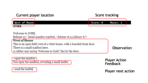
All states and actions are given in natural language. Input for the game contains more than a thousand possible actions in each state since the player can type anything.

Related Work

Text-Based Games(TBG): The state of the environment in TBG is described by simple language. The player interacts with the environment with text command which respects a pre-defined grammar. A popular example is Zork which has been tested in the paper. TBG is a good research intersection of RL and NLP, it requires language understanding, long-term memory, planning, exploration, affordability extraction, and common sense. It also often introduce stochastic dynamics to increase randomness. They highlight several open problems for RL, mainly the combinatorial and compositional properties of the action space, and game states that are only partially observable.

Representations for TBG: Good word representation is necessary in order to learn control policies from high-dimensional complex data such as text. Previous work on TBG used pre-trained embeddings directly for control, other works combined pre-trained embedding with neural networks. For example, He et al. (2015) proposed to consider an input as Bag Of Words features for a neural network, learned separately embeddings for states and actions, and then computed the Q function from autocorrelations between these embeddings.

DRL with linear function approximation: DRL methods such as the DQN have achieved state-of-the-art results in a variety of challenging, high-dimensional domains. This success is mainly because neural networks can learn rich domain representations for value function and policy. On the other hand, linear representation batch reinforcement learning methods are more stable and accurate, while feature engineering is necessary.A natural attempt at getting the best of both worlds is to learn a linear control policy on top of the representation of the last layer of a DNN. This approach was shown to refine the performance of DQNs and improve exploration. Similarly, for contextual linear bandits, Riquelme et al. showed that a neuro-linear Thompson sampling approach outperformed deep and linear bandit algorithms in practice.

RL in Large Action Spaces: Prior work concentrated on factorizing the action space into binary subspace(Pazis and Parr, 2011; Dulac-Arnold et al., 2012; Lagoudakis and Parr, 2003), other works proposed to embed the discrete actions into a continuous space, then choose the nearest discrete action according to the optimal actions in the continuous space(Dulac-Arnold et al., 2015; Van Hasselt and Wiering, 2009). He et. al. (2015)extended DQN to unbounded(natural language) action spaces. Learning to eliminate actions was first mentioned by (Even-Dar, Mannor, and Mansour, 2003). They proposed to learn confidence intervals around the value function in each state. Lipton et al.(2016a) proposed to learn a classifier that detects hazardous state and then use it to shape the reward. Fulda et al.(2017) presented a method for affordability extraction via inner products of pre-trained word embedding.

Action Elimination

The approach in the paper builds on the standard Reinforcement Learning formulation. At each time step [math]\displaystyle{ t }[/math], the agent observes state [math]\displaystyle{ s_t }[/math] and chooses a discrete action [math]\displaystyle{ a_t\in\{1,...,|A|\} }[/math]. Then, after action execution, the agent obtains a reward [math]\displaystyle{ r_t(s_t,a_t) }[/math] and observes next state [math]\displaystyle{ s_{t+1} }[/math] according to a transition kernel [math]\displaystyle{ P(s_{t+1}|s_t,a_t) }[/math]. The goal of the algorithm is to learn a policy [math]\displaystyle{ \pi(a|s) }[/math] which maximizes the expected future discounted cumulative return [math]\displaystyle{ V^\pi(s)=E^\pi[\sum_{t=0}^{\infty}\gamma^tr(s_t,a_t)|s_0=s] }[/math], where [math]\displaystyle{ 0\lt \gamma \lt 1 }[/math]. The Q-function is [math]\displaystyle{ Q^\pi(s,a)=E^\pi[\sum_{t=0}^{\infty}\gamma^tr(s_t,a_t)|s_0=s,a_0=a] }[/math], and it can be optimized by Q-learning algorithm.

After executing an action, the agent observes a binary elimination signal [math]\displaystyle{ e(s, a) }[/math] to determine which actions not to take. It equals 1 if action [math]\displaystyle{ a }[/math] may be eliminated in state [math]\displaystyle{ s }[/math] (and 0 otherwise). The signal helps mitigating the problem of large discrete action spaces. We start with the following definitions:

Definition 1:

Valid state-action pairs with respect to an elimination signal are state action pairs which the elimination process should not eliminate.

The set of valid state-action pairs contains all of the state-action pairs that are a part of some optimal policy, i.e., only strictly suboptimal state-actions can be invalid.

Definition 2:

Admissible state-action pairs with respect to an elimination algorithm are state action pairs which the elimination algorithm does not eliminate.

Definition 3:

Action Elimination Q-learning is a Q-learning algorithm which updates only admissible state-action pairs and chooses the best action in the next state from its admissible actions. We allow the base Q-learning algorithm to be any algorithm that converges to [math]\displaystyle{ Q^* }[/math] with probability 1 after observing each state-action infinitely often.

Advantages of Action Elimination

The main advantage of action elimination is that it allows the agent to overcome some of the main difficulties in large action spaces which are Function Approximation and Sample Complexity.

Function approximation: Errors in the Q-function estimates may cause the learning algorithm to converge to a suboptimal policy, this phenomenon becomes more noticeable when the action space is large. Action elimination mitigates this effect by taking the max operator only on valid actions, thus, reducing potential overestimation errors. Besides, by ignoring the invalid actions, the function approximation can also learn a simpler mapping (i.e., only the Q-values of the valid state-action pairs) leading to faster convergence and better solution.

Sample complexity: The sample complexity measures the number of steps during learning, in which the policy is not [math]\displaystyle{ \epsilon }[/math]-optimal. Assume that there are [math]\displaystyle{ A' }[/math] actions that should be eliminated and are [math]\displaystyle{ \epsilon }[/math]-optimal, i.e. their value is at least [math]\displaystyle{ V^*(s)-\epsilon }[/math]. The invalid action often returns no reward and doesn't change the state, (Lattimore and Hutter, 2012)resulting in an action gap of [math]\displaystyle{ \epsilon=(1-\gamma)V^*(s) }[/math], and this translates to [math]\displaystyle{ V^*(s)^{-2}(1-\gamma)^{-5}log(1/\delta) }[/math] wasted samples for learning each invalid state-action pair. Practically, elimination algorithm can eliminate these invalid actions and therefore speed up the learning process approximately by [math]\displaystyle{ A/A' }[/math].

Because it is difficult to embed the elimination signal into the MDP, the authors use contextual multi-armed bandits to decouple the elimination signal from the MDP, which can correctly eliminate actions when applying standard Q learning into learning process.

To embed the elimination signal, we can add an elimination penalty to shape rewards (e.g. decreasing the rewards when selecting the wrong actions). Due to the exploration of irrelevant actions during reward training/shaping, this becomes hard to tune, and slows down convergence/reduces efficiency. Another alternative is to design a policy using two interleaving signals (which are iteratively updated during policy gradient descent), maximizing the reward and minimizing the elimination signal error. This result unfortunately leads to high dependence and correlation between the two models, and each model affects the observations of the other model, which may make convergence difficult.

Action elimination with contextual bandits

Contextual bandit problem is a famous probability problem and is a natural extension from the multi-arm bandit problem.

Let [math]\displaystyle{ x(s_t)\in R^d }[/math] be the feature representation of [math]\displaystyle{ s_t }[/math]. We assume that under this representation there exists a set of parameters [math]\displaystyle{ \theta_a^*\in \mathbb{R}^d }[/math] such that the elimination signal in state [math]\displaystyle{ s_t }[/math] is [math]\displaystyle{ e_t(s_t,a) = \theta_a^{*T}x(s_t)+\eta_t }[/math], where [math]\displaystyle{ \Vert\theta_a^*\Vert_2\leq S }[/math]. [math]\displaystyle{ \eta_t }[/math] is an R-subgaussian random variable with zero mean that models additive noise to the elimination signal. When there is no noise in the elimination signal, R=0. Otherwise, [math]\displaystyle{ R\leq 1 }[/math] since the elimination signal is bounded in [0,1]. Assume the elimination signal satisfies: [math]\displaystyle{ 0\leq E[e_t(s_t,a)]\leq l }[/math] for any valid action and [math]\displaystyle{ u\leq E[e_t(s_t, a)]\leq 1 }[/math] for any invalid action. And [math]\displaystyle{ l\leq u }[/math]. Denote by [math]\displaystyle{ X_{t,a} }[/math] as the matrix whose rows are the observed state representation vectors in which action a was chosen, up to time t. [math]\displaystyle{ E_{t,a} }[/math] as the vector whose elements are the observed state representation elimination signals in which action a was chosen, up to time t. Denote the solution to the regularized linear regression [math]\displaystyle{ \Vert X_{t,a}\theta_{t,a}-E_{t,a}\Vert_2^2+\lambda\Vert \theta_{t,a}\Vert_2^2 }[/math] (for some [math]\displaystyle{ \lambda\gt 0 }[/math]) by [math]\displaystyle{ \hat{\theta}_{t,a}=\bar{V}_{t,a}^{-1}X_{t,a}^TE_{t,a} }[/math], where [math]\displaystyle{ \bar{V}_{t,a}=\lambda I + X_{t,a}^TX_{t,a} }[/math].

According to Theorem 2 in (Abbasi-Yadkori, Pal, and Szepesvari, 2011), [math]\displaystyle{ |\hat{\theta}_{t,a}^{T}x(s_t)-\theta_a^{*T}x(s_t)|\leq\sqrt{\beta_t(\delta)x(s_t)^T\bar{V}_{t,a}^{-1}x(s_t)}\ \forall t\gt 0 }[/math], where [math]\displaystyle{ \sqrt{\beta_t(\delta)}=R\sqrt{2\ \text{log}(\text{det}(\bar{V}_{t,a})^{1/2}\text{det}(\lambda I)^{-1/2}/\delta)}+\lambda^{1/2}S }[/math], with probability of at least [math]\displaystyle{ 1-\delta }[/math]. If [math]\displaystyle{ \forall s\ ,\Vert x(s)\Vert_2 \leq L }[/math], then [math]\displaystyle{ \beta_t }[/math] can be bounded by [math]\displaystyle{ \sqrt{\beta_t(\delta)} \leq R \sqrt{d\ \text{log}(1+tL^2/\lambda/\delta)}+\lambda^{1/2}S }[/math]. Next, define [math]\displaystyle{ \tilde{\delta}=\delta/k }[/math] and bound this probability for all the actions. i.e., [math]\displaystyle{ \forall a,t\gt 0 }[/math]

[math]\displaystyle{ Pr(|\hat{\theta}_{t-1,a}^{T}x(s_t)-\theta_{t-1, a}^{*T}x(s_t)|\leq\sqrt{\beta_t(\tilde\delta)x(s_t)^T\bar{V}_{t - 1,a}^{-1}x(s_t)}) \leq 1-\delta }[/math]

Recall that [math]\displaystyle{ E[e_t(s,a)]=\theta_a^{*T}x(s_t)\leq l }[/math] if a is a valid action. Then we can eliminate action a at state [math]\displaystyle{ s_t }[/math] if it satisfies:

[math]\displaystyle{ \hat{\theta}_{t-1,a}^{T}x(s_t)-\sqrt{\beta_{t-1}(\tilde\delta)x(s_t)^T\bar{V}_{t-1,a}^{-1}x(s_t)})\gt l }[/math]

with probability [math]\displaystyle{ 1-\delta }[/math] that we never eliminate any valid action. Note that [math]\displaystyle{ l, u }[/math] are not known. In practice, choosing [math]\displaystyle{ l }[/math] to be 0.5 should suffice.

Concurrent Learning

In fact, Q-learning and contextual bandit algorithms can learn simultaneously, resulting in the convergence of both algorithms, i.e., finding an optimal policy and a minimal valid action space.

If the elimination is done based on the concentration bounds of the linear contextual bandits, it can be ensured that Action Elimination Q-learning converges, as shown in Proposition 1.

Proposition 1:

Assume that all state action pairs (s,a) are visited infinitely often, unless eliminated according to [math]\displaystyle{ \hat{\theta}_{t-1,a}^Tx(s)-\sqrt{\beta_{t-1}(\tilde{\delta})x(s)^T\bar{V}_{t-1,a}^{-1}x(s))}\gt l }[/math]. Then, with a probability of at least [math]\displaystyle{ 1-\delta }[/math], action elimination Q-learning converges to the optimal Q-function for any valid state-action pairs. In addition, actions which should be eliminated are visited at most [math]\displaystyle{ T_{s,a}(t)\leq 4\beta_t/(u-l)^2 +1 }[/math] times.

Notice that when there is no noise in the elimination signal(R=0), we correctly eliminate actions with probability 1. so invalid actions will be sampled a finite number of times.

Method

The assumption that [math]\displaystyle{ e_t(s_t,a)=\theta_a^{*T}x(s_t)+\eta_t }[/math] generally does not hold when using raw features like word2vec. So the paper proposes to use the neural network's last layer as feature representation of states. A practical challenge here is that the features must be fixed over time when used by the contextual bandit. So batch-updates framework(Levine et al., 2017;Riquelme, Tucker, and Snoek, 2018) is used, where a new contextual bandit model is learned for every few steps that uses the last layer activation of the AEN as features.

Architecture of action elimination framework

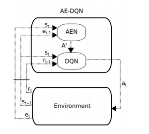
After taking action [math]\displaystyle{ a_t }[/math], the agent observes [math]\displaystyle{ (r_t,s_{t+1},e_t) }[/math]. The agent uses it to learn two function approximation deep neural networks: A DQN and an AEN. AEN provides an admissible actions set [math]\displaystyle{ A' }[/math] to the DQN, which uses this set to decide how to act and learn. The architecture for both the AEN and DQN is an NLP CNN(100 convolutional filters for AEN and 500 for DQN, with three different 1D kernels of length (1,2,3)), based on(Kim, 2014). The state is represented as a sequence of words, composed of the game descriptor and the player's inventory. These are truncated or zero padded to a length of 50 descriptor + 15 inventory words and each word is embedded into continuous vectors using word2vec in [math]\displaystyle{ R^{300} }[/math]. The features of the last four states are then concatenated together such that the final state representations s are in [math]\displaystyle{ R^{78000} }[/math]. The AEN is trained to minimize the MSE loss, using the elimination signal as a label. The code, the Zork domain, and the implementation of the elimination signal can be found here.

Psuedocode of the Algorithm

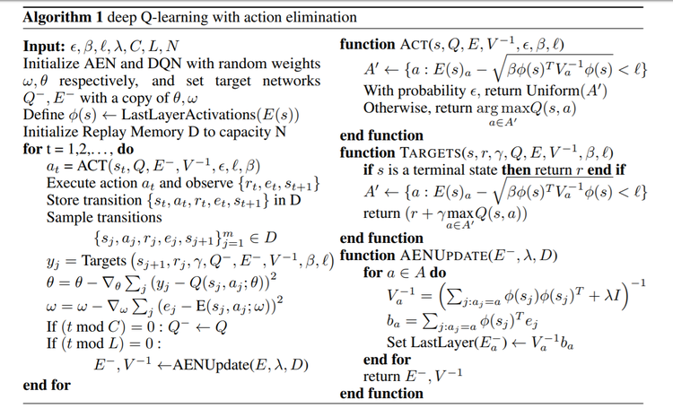
AE-DQN trains two networks: a DQN denoted by Q and an AEN denoted by E. The algorithm creates a linear contextual bandit model from it every L iterations with procedure AENUpdate(). This procedure uses the activations of the last hidden layer of E as features, which are then used to create a contextual linear bandit model.AENUpdate() then solved this model and plugin it into the target AEN. The contextual linear bandit model [math]\displaystyle{ (E^-,V) }[/math] is then used to eliminate actions via the ACT() and Target() functions. ACT() follows an [math]\displaystyle{ \epsilon }[/math]-greedy mechanism on the admissible actions set. For exploitation, it selects the action with highest Q-value by taking an argmax on Q-values among [math]\displaystyle{ A' }[/math]. For exploration, it selects an action uniformly from [math]\displaystyle{ A' }[/math]. The targets() procedure is estimating the value function by taking max over Q-values only among admissible actions, hence, reducing function approximation errors.

Experiments

Grid Domain

The authors start by evaluating our algorithm on a small grid world domain with 9 rooms, where they ca analyze the effect of the action elimination (visualization can be found in the appendix). In this domain, the agent starts at the center of the grid and needs to navigate to its upper-left corner. On every step, the agent suffers a penalty of (−1), with a terminal reward of 0. Prior to the game, the states are randomly divided into K categories. The environment has 4K navigation actions, 4 for each category, each with a probability to move in a random direction. If the chosen action belongs to the same category as the state, the action is performed correctly in probability pTc = 0.75. Otherwise, it will be performed correctly in probability pFc = 0.5. If the action does not fit the state category, the elimination signal equals 1, and if the action and state belong to the same category, then e = 0. The optimal policy will only use the navigation actions from the same type as the state, and all of the other actions are strictly suboptimal. A basic comparison between vanilla Q-learning without action elimination (green) and a tabular version of the action elimination Q-learning (blue) can be found in the figure below. In all of the figures, the results are compared to the case with one category (red), i.e., only 4 basic navigation actions, which forms an upper bound on performance with multiple categories. In Figure (a),(c), the episode length is T = 150, and in Figure (b) it is T = 300, to allow sufficient exploration for the vanilla Q-Learning. It is clear from the simulations that the action elimination dramatically improves the results in large action spaces. Also, note that the gain from action elimination increases with the grid size since the elimination allows the agent to reach the goal earlier.

Performance of agents in grid world

Zork domain

The world of Zork presents a rich environment with a large state and action space. Zork players describe their actions using natural language instructions. For example, "open the mailbox". Then their actions were processed by a sophisticated natural language parser. Based on the results, the game presents the outcome of the action. The goal of Zork is to collect the Twenty Treasures of Zork and install them in the trophy case. Points that are generated from the game's scoring system are given to the agent as the reward. For example, the player gets the points when solving the puzzles. Placing all treasures in the trophy will get 350 points. The elimination signal is given in two forms, "wrong parse" flag, and text feedback "you cannot take that". These two signals are grouped together into a single binary signal which then provided to the algorithm.

Left:the world of Zork.Right:subdomains of Zork.

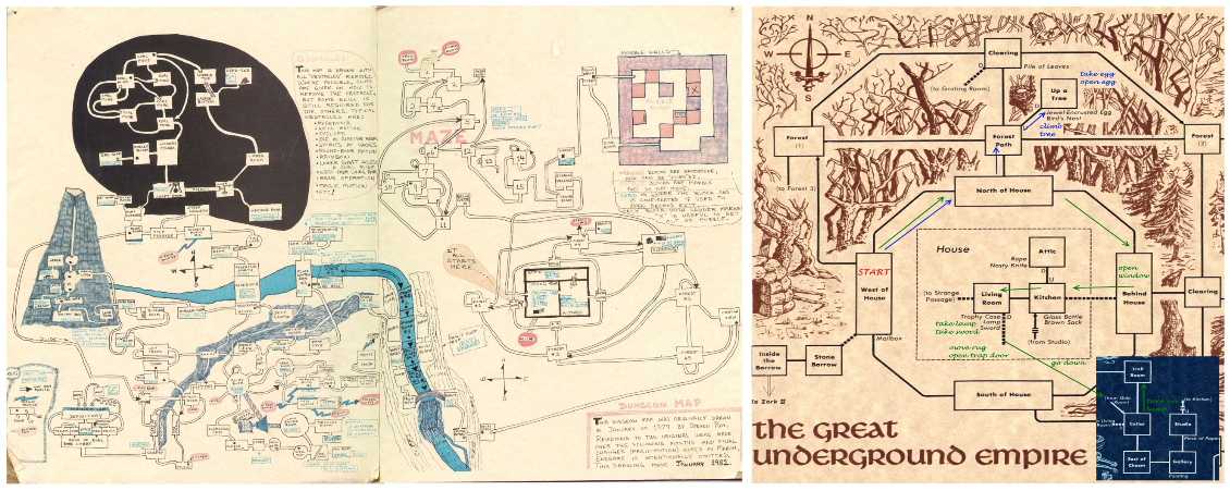
Experiments begin with the two subdomains of Zork domains: Egg Quest and the Troll Quest. For these subdomains, an additional reward signal is provided to guide the agent towards solving specific tasks and make the results more visible. A reward of -1 is applied at every time step to encourage the agent to favor short paths. Each trajectory terminates is upon completing the quest or after T steps are taken. The discounted factor for training is [math]\displaystyle{ \gamma=0.8 }[/math] and [math]\displaystyle{ \gamma=1 }[/math] during evaluation. Also [math]\displaystyle{ \beta=0.5, l=0.6 }[/math] in all experiments.

Egg Quest

The goal for this quest is to find and open the jewel-encrusted egg hidden on a tree in the forest. An egg-splorer goes on an adventure to find a mystical ancient relic with his furry companion. You can have a look at the game at EggQuest

The agent will get 100 points upon completing this task. For action space, there are 9 fixed actions for navigation, and a second subset which consisting [math]\displaystyle{ N_{Take} }[/math] actions for taking possible objects in the game. [math]\displaystyle{ N_{Take}=200 (set A_1), N_{Take}=300 (set A_2) }[/math] has been tested separately. AE-DQN (blue) and a vanilla DQN agent (green) has been tested in this quest.

Performance of agents in the egg quest.

Figure a) corresponds to the set [math]\displaystyle{ A_1 }[/math], with T=100, b) corresponds to the set [math]\displaystyle{ A_2 }[/math], with T=100, and c) corresponds to the set [math]\displaystyle{ A_2 }[/math], with T=200. Both agents have performed well on sets a and c. However, the AE-DQN agent has learned much faster than the DQN on set b, which implies that action elimination is more robust to hyperparameter optimization when the action space is large. One important observation to note is that the three figures have different scales for the cumulative reward. While the AE-DQN outperformed the standard DQN in figure b, both models performed significantly better with the hyperparameter configuration in figure c.

Troll Quest

The goal of this quest is to find the troll. To do it the agent needs to find the way to the house, use a lantern to expose the hidden entrance to the underworld. It will get 100 points upon achieving the goal. This quest is a larger problem than Egg Quest. The action set [math]\displaystyle{ A_1 }[/math] is 200 take actions and 15 necessary actions, 215 in total.

Results in the Troll Quest.

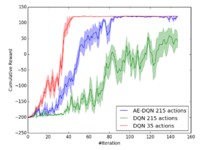
The red line above is an "optimal elimination" baseline which consists of only 35 actions(15 essential and 20 relevant take actions). We can see that AE-DQN still outperforms DQN and its improvement over DQN is more significant in the Troll Quest than the Egg quest. Also, it achieves compatible performance to the "optimal elimination" baseline.

Open Zork

Lastly, the "Open Zork" domain has been tested which only the environment reward has been used. 1M steps have been trained. Each trajectory terminates after T=200 steps. Two action sets have been used:[math]\displaystyle{ A_3 }[/math], the "Minimal Zork" action set, which is the minimal set of actions (131) that is required to solve the game. [math]\displaystyle{ A_4 }[/math], the "Open Zork" action set (1227) which composed of {Verb, Object} tuples for all the verbs and objects in the game.

[[]]

Results in "Open Zork".

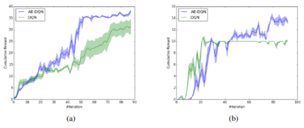
The above Figure shows the learning curve for both AE-DQN and DQN. We can see that AE-DQN (blue) still outperform the DQN (blue) in terms of speed and cumulative reward.

Conclusion

In this paper, the authors proposed a Deep Reinforcement Learning model for sub-optimal actions while performing Q-learning. Moreover, they showed that by eliminating actions, using linear contextual bandits with theoretical guarantees of convergence, the size of the action space is reduced, exploration is more effective, and learning is improved when tested on Zork, a text-based game.

For future work the authors aim to investigate more sophisticated architectures and tackle learning shared representations for elimination and control which may boost performance on both tasks.

They also hope to to investigate other mechanisms for action elimination, such as eliminating actions that result from low Q-values as in Even-Dar, Mannor, and Mansour, 2003.

The authors also hope to generate elimination signals in real-world domains and achieve the purpose of eliminating the signal implicitly.

Critique

The paper is not a significant algorithmic contribution and it merely adds an extra layer of complexity to the very famous DQN algorithm. All the experimental domains considered in the paper are discrete action problems that have so many actions that it could have been easily extended to a continuous action problem. In continuous action space there are several policy gradient based RL algorithms that have provided stronger performances. The authors should have ideally compared their methods to such algorithms like PPO or DRPO.

Even with the critique above, the paper presents mathematical/theoretical justifications of the methodology. Moreover, since the methodology is built on the standard RL framework, this means that other variant RL algorithms can apply the idea to decrease the complexity and increase the performance. Moreover, the there are some rooms for applying technical variations for the algorithm.

Also, since we are utilizing the system's response to irrelevant actions, an intuitive approach to eliminate such irrelevant actions is to add a huge negative reward for such actions, which will be much easier than the approach suggested by this paper. However, the in experiments, the author only compares AE-DQN to traditional DQN, not traditional DQN with negative rewards assigned to irrelevant actions.

After all, the name that the authors have chosen is a good and attractive choice and matches our brain's structure which in so many real-world scenarios detects what not to learn.

Reference

1. Chu, W.; Li, L.; Reyzin, L.; and Schapire, R. 2011. Contextual bandits with linear payoff functions. In Proceedings of the Fourteenth International Conference on Artificial Intelligence and Statistics.

2. Côté,M.-A.;Kádár,Á.;Yuan,X.;Kybartas,B.;Barnes,T.;Fine,E.;Moore,J.;Hausknecht,M.;Asri, L. E.; Adada, M.; et al. 2018. Textworld: A learning environment for text-based games. arXiv.

3. Dulac-Arnold, G.; Evans, R.; van Hasselt, H.; Sunehag, P.; Lillicrap, T.; Hunt, J.; Mann, T.; Weber, T.; Degris, T.; and Coppin, B. 2015. Deep reinforcement learning in large discrete action spaces. arXiv.

4. He, J.; Chen, J.; He, X.; Gao, J.; Li, L.; Deng, L.; and Ostendorf, M. 2015. Deep reinforcement learning with an unbounded action space. CoRR abs/1511.04636.

5. Kim, Y. 2014. Convolutional neural networks for sentence classification. arXiv preprint.

6. VanHasselt,H.,andWiering,M.A. 2009. Usingcontinuousactionspacestosolvediscreteproblems. In Neural Networks, 2009. IJCNN 2009. International Joint Conference on, 1149–1156. IEEE.

7. Watkins, C. J., and Dayan, P. 1992. Q-learning. Machine learning 8(3-4):279–292.

8. Su, P.-H.; Gasic, M.; Mrksic, N.; Rojas-Barahona, L.; Ultes, S.; Vandyke, D.; Wen, T.-H.; and Young, S. 2016. Continuously learning neural dialogue management. arXiv preprint.

9. Wu, Y.; Schuster, M.; Chen, Z.; Le, Q. V.; Norouzi, M.; Macherey, W.; Krikun, M.; Cao, Y.; Gao, Q.; Macherey, K.; et al. 2016. Google’s neural machine translation system: Bridging the gap between human and machine translation. arXiv preprint.

10. Yuan, X.; Côté, M.-A.; Sordoni, A.; Laroche, R.; Combes, R. T. d.; Hausknecht, M.; and Trischler, A. 2018. Counting to explore and generalize in text-based games. arXiv preprint arXiv:1806.1152

11. Zahavy, T.; Haroush, M.; Merlis, N.; Mankowitz, D. J.; 2018. Learn What Not to Learn: Action Elimination with Deep Reinforcement Learning.