ShakeDrop Regularization

Introduction

Current state of the art techniques for object classification are deep neural networks based on the residual block, first published by (He et al., 2016). This technique has been the foundation of several improved networks, including Wide ResNet (Zagoruyko & Komodakis, 2016), PyramdNet (Han et al., 2017) and ResNeXt (Xie et al., 2017). They have been further improved by regularization, such as Stochastic Depth (ResDrop) (Huang et al., 2016) and Shake-Shake (Gastaldi, 2017). Shake-Shake applied to ResNext has achieved one of the lowest error rates on the CIFAR-10 and CIFAR-100 datasets. However, it is only applicable to multi branch architectures, and is not memory efficient. This paper seeks to formulate a general expansion of Shake-Shake that can be applied to any residual block based network.

Existing Methods

Deep Approaches

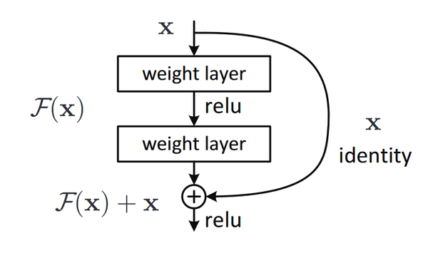
ResNet, was the first use of residual blocks, a foundational feature in many modern state of the art convolution neural networks. They can be formulated as [math]\displaystyle{ G(x) = x + F(x) }[/math] where x and G(x) are the input and output of the residual block, and [math]\displaystyle{ F(x) }[/math] is the output of the residual block. A residual block typically performs a convolution operation and then passes the result plus its input onto the next block.

An example of a simple residual block from Deep Residual Learning for Image Recognition by He et al. 2016

ResNet is constructed out of a large number of these residual blocks sequentially stacked.

PyramidNet is an important iteration that built on ResNet and WideResNet by gradually increasing channels on each residual block. The residual block is similar to those used in ResNet. It has been use to generate some of the first successful convolution neural networks with very large depth, at 272 layers. Amongst unmodified network architectures, it performs the best on the CIFAR datasets.

Non-Deep Approaches

Wide ResNet modified ResNet by increasing channels in each layer, having a wider and shallower structure. Similarly to PyramidNet, this architecture avoids some of the pitfalls in the orginal formulation of ResNet.

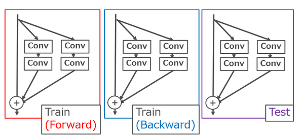
ResNeXt achieved performance beyond that of Wide ResNet with only a small increase in the number of parameters. It can be formulated as [math]\displaystyle{ G(x) = x + F_1(x)+F_2(x) }[/math]. In this case, [math]\displaystyle{ F_1(x) }[/math] and [math]\displaystyle{ F_2(x) }[/math] are the outputs of two paired convolution operations in a single residual block. The number of branches is not limited to 2, and will control the result of this network.

Simplified ResNeXt Convolution Block

Regularization Methods

Stochastic Depth helped address the issue of vanishing gradients in ResNet. It works by randomly dropping residual blocks. On the [math]\displaystyle{ l^th }[/math] residual block the Stochastic Depth process is given as [math]\displaystyle{ G(x)=x+b_lF(x) }[/math] where [math]\displaystyle{ b_l \in {0,1} }[/math] is a Bernoulli random variable with probability [math]\displaystyle{ p_l }[/math]. Using a constant value for [math]\displaystyle{ p_l }[/math] didn't work well, so instead a linear decay rule [math]\displaystyle{ p_l = 1 - \frac{l}{L}(1-p_L) }[/math] was used. In this equation, [math]\displaystyle{ L }[/math] is the number of layers, and [math]\displaystyle{ p_L }[/math] is the initial parameter.

Shake-Shake is a regularization method that specifically improves the ResNeXt architecture. It can be given as [math]\displaystyle{ G(x)=x+\alpha F_1(x)+(1-\alpha)F_2(x) }[/math], where [math]\displaystyle{ \alpha \in [0,1] }[/math] is a random coefficient. [math]\displaystyle{ \alpha }[/math] is used during the forward pass, and another identically distributed random parameter [math]\displaystyle{ \beta }[/math] is used in the backward pass. This caused one of the two paired convolution operations to be dropped, and further improved ResNeXt.

Proposed Method

This paper seeks to generalize the method proposed in Shake-Shake to be applied to any residual structure network. Shake-Shake. The initial formulation of 1-branch shake is [math]\displaystyle{ G(x) = x + \alpha F(x) }[/math]. In this case, [math]\displaystyle{ \alpha }[/math] is a coefficient that disturbs the forward pass, but is not necessarily constrained to be [0,1]. Another corresponding coefficient [math]\displaystyle{ \beta }[/math] is used in the backwards pass. Applying this simple adaptation of Shake-Shake on a 110-layer version of PyramidNet with [math]\displaystyle{ \alpha \in [0,1] }[/math] and [math]\displaystyle{ \beta \in [0,1] }[/math] performs abysmally, with an error rate of 77.99%.

This failure is a result of the setup causing too much perturbation. A trick is needed to promote learning with large perturbations, to preserve the regularization effect. The idea of the authors is to borrow from ResDrop and combine that with Shake-Shake. This works by randomly deciding whether to apply 1-branch shake. This in creates in effect two networks, the original network without a regularization component, and a regularized network. When the non regularized network is selected, learning is promoted, when the perturbed network is selected, learning is disturbed. Achieving good performance requires a balance between the two.

ShakeDrop is given as

[math]\displaystyle{ G(x) = x + (b_l + \alpha - b_l \alpha)F(x) }[/math],

where [math]\displaystyle{ b_l }[/math] is a Bernoulli random variable following the linear decay rule used in Stochastic Depth. An alternative presentation is

[math]\displaystyle{ G(x) = x + F(x) }[/math] if [math]\displaystyle{ b_l = 1 }[/math]

[math]\displaystyle{ G(x) = x + \alpha F(x) }[/math] otherwise.

If [math]\displaystyle{ b_l = 1 }[/math] then ShakeDrop is equivalent to the original network, otherwise it is the network + 1-branch Shake. Regardless of the value of [math]\displaystyle{ \beta }[/math] on the backwards pass, the network weights will be updated.

References

[He et al., 2016] Kaiming He, Xiangyu Zhang, Shaoqing Ren, and Jian Sun. Deep residual learning for image recognition. In Proc. CVPR, 2016.

[Zagoruyko & Komodakis, 2016] Sergey Zagoruyko and Nikos Komodakis. Wide residual networks. In Proc. BMVC, 2016.

[Han et al., 2017] Dongyoon Han, Jiwhan Kim, and Junmo Kim. Deep pyramidal residual networks. In Proc. CVPR, 2017a.

[Xie et al., 2017] Saining Xie, Ross Girshick, Piotr Dollar, Zhuowen Tu, and Kaiming He. Aggregated residual transformations for deep neural networks. In Proc. CVPR, 2017.

[Huang et al., 2016] Gao Huang, Yu Sun, Zhuang Liu, Daniel Sedra, and Kilian Weinberger. Deep networks with stochastic depth. arXiv preprint arXiv:1603.09382v3, 2016.

[Gastaldi, 2017] Xavier Gastaldi. Shake-shake regularization. arXiv preprint arXiv:1705.07485v2, 2017.