Deep Reinforcement Learning in Continuous Action Spaces a Case Study in the Game of Simulated Curling

This page provides a summary and critique of the paper Deep Reinforcement Learning in Continuous Action Spaces: a Case Study in the Game of Simulated Curling [Online Source], published in ICML 2018. The source code for this paper is available here

Introduction and Motivation

In recent years, Reinforcement Learning methods have been applied to many different games, such as chess and checkers. More recently, the use of CNN's has allowed neural networks to out-perform humans in many difficult games, such as Go. However, many of these cases involve a discrete state or action space; the number of actions a player can take and/or the number of possible game states are finite.

Interacting with the real world (e.g.; a scenario that involves moving physical objects) typically involves working with a continuous action space. It is thus important to develop strategies for dealing with continuous action spaces. Deep neural networks that are designed to succeed in finite action spaces are not necessarily suitable for continuous action space problems. This is due to the fact that deterministic discretization of a continuous action space causes strong biases in policy evaluation and improvement.

This paper introduces a method to allow learning with continuous action spaces. A CNN is used to perform learning on a discretion state and action spaces, and then a continuous action search is performed on these discrete results.

Curling is chosen as a domain to test the network on. Curling was chosen due to its large action space, potential for complicated strategies, and need for precise interactions.

Curling

Curling is a sport played by two teams on a long sheet of ice. Roughly, the goal is for each time to slide rocks closer to the target on the other end of the sheet than the other team. The next sections will provide a background on the game play, and potential challenges/concerns for learning algorithms. A terminology section follows.

Game play

A game of curling is divided into ends. In each end, players from both teams alternate throwing (sliding) eight rocks to the other end of the ice sheet, known as the house. Rocks must land in a certain area in order to stay in play, and must touch or be inside concentric rings (12ft diameter and smaller) in order to score points. At the end of each end, the team with rocks closest to the center of the house scores points.

When throwing a rock, the curling can spin the rock. This allows the rock to 'curl' its path towards the house and can allow rocks to travel around other rocks. Team members are also able to sweep the ice in front of a moving rock in order to decrease friction, which allows for fine-tuning of distance (though the physics of sweeping are not implemented in the simulation used).

Curling offers many possible high-level actions, which are directed by a team member to the throwing member. An example set of these includes:

• Draw: Throw a rock to a target location
• Freeze: Draw a rock up against another rock
• Takeout: Knock another rock out of the house. Can be combined with different ricochet directions
• Guard: Place a rock in front of another, to block other rocks (ex: takeouts)

Challenges for AI

Curling offers many challenges for curling based on its physics and rules. This section lists a few concerns.

The effect of changing actions can be highly nonlinear and discontinuous. This can be seen when considering that a 1-cm deviation in a path can make the difference between a high-speed collision, or lack of collision.

Curling will require both offensive and defensive strategies. For example, consider the fact that the last team to throw a rock each end only needs to place that rock closer than the opposing team's rocks to score a point and invalidate any opposing rocks in the house. The opposing team should thus be considering how to prevent this from happening, in addition to scoring points themselves.

Curling also has a concept known as 'the hammer'. The hammer belongs to the team which throws the last rock each end, providing an advantage, and is given to the team that does not score points each end. It could very well be a good strategy to try not to win a single point in an end (if already ahead in points, etc), as this would give the advantage to the opposing team.

Finally, curling has a rule known as the 'Free Guard Zone'. This applies to the first 4 rocks thrown (2 from each team). If they land short of the house, but still in play, then the rocks are not allowed to be removed (via collisions) until all of the first 4 rocks have been thrown.

Terminology

• End: A round of the game
• House: The end of the sheet of ice, which contains
• Hammer: The team that throws the last rock of an end 'has the hammer'
• Hog Line: thick line that is drawn in front of the house, orthogonal to the length of the ice sheet. Rocks must pass this line to remain in play.
• Back Line: think line drawn just behind the house. Rocks that pass this line are removed from play.

Related Work

AlphaGo Lee

AlphaGo Lee (Silver et al., 2016, [5]) refers to an algorithm used to play the game Go, which was able to defeat international champion Lee Sedol.

Go game:

• Start with 19x19 empty board
• One player take black stones and the other take white stones
• Two players take turns to put stones on the board
• Rules:

  1. If one connected part is completely surrounded by the opponents stones, remove it from the board

  2. Ko rule: Forbids a board play to repeat a board position

• End when there is no valuable moves on the board.
• Count the territory of both players.
• Add 7.5 points to whites points (called Komi).

Two neural networks were trained on the moves of human experts, to act as both a policy network and a value network. A Monte Carlo Tree Search algorithm was used for policy improvement.

The AlphaGo Lee policy network predicts the best move given a board configuration. It has a CNN architecture with 13 hidden layers, and it is trained using expert game play data and improved through self-play.

The value network evaluates the probability of winning given a board configuration. It consists of a CNN with 14 hidden layers, and it is trained using self-play data from the policy network.

Finally, the two networks are combined using Monte-Carlo Tree Search, which performs look ahead search to select the actions for game play.

The use of both policy and value networks are reflected in this paper's work.

AlphaGo Zero

AlphaGo Zero (Silver et al., 2017, [6]) is an improvement on the AlphaGo Lee algorithm. AlphaGo Zero uses a unified neural network in place of the separate policy and value networks and is trained on self-play, without the need of expert training.

The unification of networks and self-play are also reflected in this paper.

Curling Algorithms

Some past algorithms have been proposed to deal with continuous action spaces. For example, (Yammamoto et al, 2015, [7]) use game tree search methods in a discretized space. The value of an action is taken as the average of nearby values, with respect to some knowledge of execution uncertainty.

Monte Carlo Tree Search

Monte Carlo Tree Search algorithms have been applied to continuous action spaces. These algorithms, to be discussed in further detail, balance exploration of different states, with knowledge of paths of execution through past games. An MCTS called [math]\displaystyle{ KR-UCT }[/math] which is able to find effective selections and use kernel regression (KR) and kernel density estimation(KDE) to estimate rewards using neighborhood information has been applied to continuous action space by researchers.

With bandit problem, scholars used hierarchical optimistic optimization(HOO) to create a cover tree and divide the action space into small ranges at different depths, where the most promising node will create fine granularity estimates.

Curling Physics and Simulation

Several references in the paper refer to the study and simulation of curling physics. Scholars have analyzed friction coefficients between curling stones and ice. While modelling the changes in friction on ice is not possible, a fixed friction coefficient was predefined in the simulation. The behavior of the stones was also modeled. Important parameters are trained from professional players. The authors used the same parameters in this paper.

General Background of Algorithms

Policy and Value Functions

A policy function is trained to provide the best action to take, given a current state. Policy iteration is an algorithm used to improve a policy over time. This is done by alternating between policy evaluation and policy improvement.

POLICY IMPROVEMENT: LEARNING ACTION POLICY

Action policy [math]\displaystyle{ p_{\sigma}(a|s) }[/math] outputs a probability distribution over all eligible moves [math]\displaystyle{ a }[/math]. Here [math]\displaystyle{ \sigma }[/math] denotes the weights of a neural network that approximates the policy. [math]\displaystyle{ s }[/math] denotes the set of states and [math]\displaystyle{ a }[/math] denotes the set of actions taken in the environment. The policy is a function that returns a action given the state at which the agent is present. We can use policy gradient reinforcement learning to train action policy. It is updated by stochastic gradient ascent in the direction that maximizes the expected outcome at each time step t, \[ \Delta \rho \propto \frac{\partial p_{\rho}(a_t|s_t)}{\partial \rho} r(s_t) \] where [math]\displaystyle{ r(s_t) }[/math] is the return.

POLICY EVALUATION: LEARNING VALUE FUNCTIONS

A value function is trained to estimate the value of a value of being in a certain state with parameter [math]\displaystyle{ \theta }[/math]. It is trained based on records of state-action-reward sets [math]\displaystyle{ (s, r(s)) }[/math] by using stochastic gradient de- scent to minimize the mean squared error (MSE) between the predicted regression value and the corresponding outcome, \[ \Delta \theta \propto \frac{\partial v_{\theta}(s)}{\partial \theta}(r(s)-v_{\theta}(s)) \]

Monte Carlo Tree Search

Monte Carlo Tree Search (MCTS) is a search algorithm used for finite-horizon tasks (ex: in curling, only 16 moves, or throw stones, are taken each end).

MCTS is a tree search algorithm similar to minimax. However, MCTS is probabilistic and does not need to explore a full game tree or even a tree reduced with alpha-beta pruning. This makes it tractable for games such as GO, and curling.

Nodes of the tree are game states, and branches represent actions. Each node stores statistics on how many times it has been visited by the MCTS, as well as the number of wins encountered by playouts from that position. A node has been considered 'visited' if a full playout has started from that node. A node is considered 'expanded' if all its children have been visited.

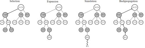
MCTS begins with the selection phase, which involves traversing known states/actions. This involves expanding the tree by beginning at the root node, and selecting the child/score with the highest 'score'. From each successive node, a path down to a root node is explored in a similar fashion.

The next phase, expansion, begins when the algorithm reaches a node where not all children have been visited (ie: the node has not been fully expanded). In the expansion phase, children of the node are visited, and simulations run from their states.

Once the new child is expanded, simulation takes place. This refers to a full playout of the game from the point of the current node, and can involve many strategies, such as randomly taken moves, the use of heuristics, etc.

The final phase is update or back-propagation (unrelated to the neural network algorithm). In this phase, the result of the simulation (ie: win/lose) is update in the statistics of all parent nodes.

A selection function known as Upper Confidence Bound (UCT) can be used for selecting which node to select. The formula for this equation is shown below [source]. Note that the first term essentially acts as an average score of games played from a certain node. The second term, meanwhile, will grow when sibling nodes are expanded. This means that unexplored nodes will gradually increase their UCT score, and be selected in the future.

[math]\displaystyle{ \frac{w_i}{n_i} + c \sqrt{\frac{\ln t}{n_i}} }[/math]

In which

• [math]\displaystyle{ w_i = }[/math] number of wins after [math]\displaystyle{ i }[/math]th move
• [math]\displaystyle{ n_i = }[/math] number of simulations after [math]\displaystyle{ i }[/math]th move
• [math]\displaystyle{ c = }[/math] exploration parameter (theoritically eqal to [math]\displaystyle{ \sqrt{2} }[/math])
• [math]\displaystyle{ t = }[/math] total number of simulations for the parent node

Sources: 2,3,4

Kernel Regression

Kernel regression is a form of weighted averaging which uses a kernel function as a weight to estimate the conditional expectation of a random variable. Given two items of data, x, each of which has a value y associated with them, and a choice of Kernel K, the kernel functions outputs a weighting factor. An estimate of the value of a new, unseen point, is then calculated as the weighted average of values of surrounding points.

A typical kernel is a Gaussian kernel, shown below. The formula for calculating estimated value is shown below as well (sources: Lee et al.).

The denominator of the conditional expectation is related to kernel density estimation, which is defined as [math]\displaystyle{ W(x)=\sum_{i=0}^n K(x,x_i) }[/math].

In this case, the combination of the two-act to weigh scores of samples closest to x more strongly.

Methods

Variable Definitions

The following variables are used often in the paper:

• [math]\displaystyle{ s }[/math]: A state in the game, as described below as the input to the network.
• [math]\displaystyle{ s_t }[/math]: The state at a certain time-step of the game. Time-steps refer to full turns in the game
• [math]\displaystyle{ a_t }[/math]: The action taken in state [math]\displaystyle{ s_t }[/math]
• [math]\displaystyle{ A_t }[/math]: The actions taken for sibling nodes related to [math]\displaystyle{ a_t }[/math] in MCTS
• [math]\displaystyle{ n_{a_t} }[/math]: The number of visits to node a in MCTS
• [math]\displaystyle{ v_{a_t} }[/math]: The MCTS value estimate of a node

Network Design

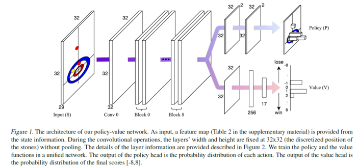
The authors design a CNN called the 'policy-value' network. The network consists of a common network structure, which is then split into 'policy' and 'value' outputs. This network is trained to learn a probability distribution of actions to take, and expected rewards, given an input state.

Shared Structure

The network consists of 1 convolutional layer followed by 9 residual blocks, each block consisting of 2 convolutional layers with 32 3x3 filters. The structure of this network is shown below:

Figure 2. A detail description of our policy-value network. The shared network is composed of one convolutional layer and nine residual blocks. Each residual block (explained in b) has two convolutional layer with batch normalization (Ioffe & Szegedy, 2015[11]) followed by the addition of the input and the residual block. Each layer in the shared network uses 3x3 filters. The policy head has two more convolutional layers, while the value head has two fully connected layers on top of a convolutional layer. For the activation function of each convolutional layer, ReLU (Nair & Hinton[12]) is used.

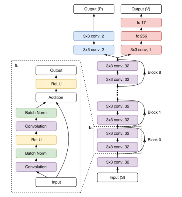
the input to this network is the following:

• Location of stones
• Order to tee (the center of the sheet)
• A 32x32 grid of representation of the ice sheet, representing which stones are present in each grid cell.

The authors do not describe how the stone-based information is added to the 32x32 grid as input to the network.

Policy Network

The policy head is created by adding 2 convolutional layers with 2 (two) 3x3 filters to the main body of the network. The output of the policy head is a distribution of probabilities of the actions to select the best shot out of a 32x32x2 set of actions. The actions represent target locations in the grid and spin direction of the stone.

Value Network

The valve head is created by adding a convolution layer with 1 3x3 filter, and dense layers of 256 and 17 units, to the shared network. The 17 output units represent a probability of scores in the range of [-8,8], which are the possible scores at each end of a curling game.

Continuous Action Search

The policy head of the network only outputs actions from a discretized action space. For real-life interactions, and especially in curling, this will not suffice, as very fine adjustments to actions can make significant differences in outcomes.

Actions in the continuous space are generated using an MCTS algorithm, with the following steps:

Selection

From a given state, the list of already-visited actions is denoted as A_t. Scores and the number of visits to each node are estimated using the equations below (the first equation shows the expectation of the end value for one-end games). These are likely estimated rather than simply taken from the MCTS statistics to help account for the differences in a continuous action space.

The UCB formula is then used to select an action to expand.

The actions that are taken in the simulator appear to be drawn from a Gaussian centered around [math]\displaystyle{ a_t }[/math]. This allows exploration in the continuous action space.

Expansion

The authors use a variant of regular UCT for expansion. In this case, they expand a new node only when existing nodes have been visited a certain number of times. The authors utilize a widening approach to overcome problems with standard UCT performing a shallow search when there is a large action space.

Simulation

Instead of simulating with a random game playout, the authors use the value network to estimate the likely score associated with a state. This speeds up simulation (assuming the network is well trained), as the game does not actually need to be simulated.

Backpropogation

Standard backpropagation is used, updating both the values and number of visits stored in the path of parent nodes.

Supervised Learning

During supervised training, data is gathered from the program AyumuGAT'16 ([8]). This program is also based on both an MCTS algorithm, and a high-performance AI curling program. 400 000 state-action pairs were generated during this training.

Policy Network

The policy network was trained to learn the action taken in each state. Here, the likelihood of the taken action was set to be 1, and the likelihood of other actions to be 0.

Value Network

The value network was trained by 'd-depth simulations and bootstrapping of the prediction to handle the high variance in rewards resulting from a sequence of stochastic moves' (quote taken from paper). In this case, m state-action pairs were sampled from the training data. For each pair, [math]\displaystyle{ (s_t, a_t) }[/math], a state d' steps ahead was generated, [math]\displaystyle{ s_{t+d} }[/math]. This process dealt with uncertainty by considering all actions in this rollout to have no uncertainty, and allowing uncertainty in the last action, a_t+d-1. The value network is used to predict the value for this state, [math]\displaystyle{ z_t }[/math], and the value is used for learning the value at s_t.

Policy-Value Network

The policy-value network was trained to maximize the similarity of the predicted policy and value, and the actual policy and value from a state. The learning algorithm parameters are:

• Algorithm: stochastic gradient descent
• Batch size: 256
• Momentum: 0.9
• L2 regularization: 0.0001
• Training time: ~100 epochs
• Learning rate: initialized at 0.01, reduced twice

A multi-task loss function was used. This takes the summation of the cross-entropy losses of each prediction:

Self-Play Reinforcement Learning

After initialization by supervised learning, the algorithm uses self-play to further train itself. During this training, the policy network learns probabilities from the MCTS process, while the value network learns from game outcomes.

At a game state s_t:

1) the algorithm outputs a prediction z_t. This is en estimate of game score probabilities. It is based on similar past actions, and computed using kernel regression.

2) the algorithm outputs a prediction [math]\displaystyle{ \pi_t }[/math], representing a probability distribution of actions. These are proportional to estimated visit counts from MCTS, based on kernel density estimation.

It is not clear how these predictions are created. It would seem likely that the policy-value network generates these, but the wording of the paper suggests they are generated from MCTS statistics.

The policy-value network is updated by sampling data [math]\displaystyle{ (s, \pi, z) }[/math] from recent history of self-play. The same loss function is used as before.

It is not clear how the improved network is used, as MCTS seems to be the driving process at this point.

Long-Term Strategy Learning

Finally, the authors implement a new strategy to augment their algorithm for long-term play. In this context, this refers to playing a game over many ends, where the strategy to win a single end may not be a good strategy to win a full game. For example, scoring one point in an end, while being one point ahead, gives the advantage to the other team in the next round (as they will throw the last stone). The other team could then use the advantage to score two points, taking the lead.

The authors build a 'winning percentage' table. This table stores the percentage of games won, based on the number of ends left, and the difference in score (current team - opposing team). This can be computed iteratively and using the probability distribution estimation of one-end scores.

Final Algorithms

The authors make use of the following versions of their algorithm:

KR-DL

Kernel regression-deep learning: This algorithm is trained only by supervised learning.

KR-DRL

Kernel regression-deep reinforcement learning: This algorithm is trained by supervised learning (ie: initialized as the KR-DL algorithm), and again on self-play. During self-play, each shot is selected after 400 MCTS simulations of k=20 randomly selected actions. Data for self-play was collected over a week on 5 GPUS and generated 5 million game positions. The policy-value network was continually updated using samples from the latest 1 million game positions.

KR-DRL-MES

Kernel regression-deep reinforcement learning-multi-ends-strategy: This algorithm makes use of the winning percentage table generated from self-play.

Testing and Results

The authors use data from the public program AyumuGAT’16 to test. Testing is done with a simulated curling program [9]. This simulator does not deal with changing ice conditions, or sweeping, but does deal with stone trajectories and collisions.

Comparison of KR-DL-UCT and DL-UCT

The first test compares an algorithm trained with kernel regression with an algorithm trained without kernel regression, to show the contribution that kernel regression adds to the performance. Both algorithms have networks initialised with the supervised learning, and then trained with two different algorithms for self-play. KR-DL-UCT uses the algorithm described above. The authors do not go into detail on how DL-UCT selects shots, but state that a constant is set to allow exploration.

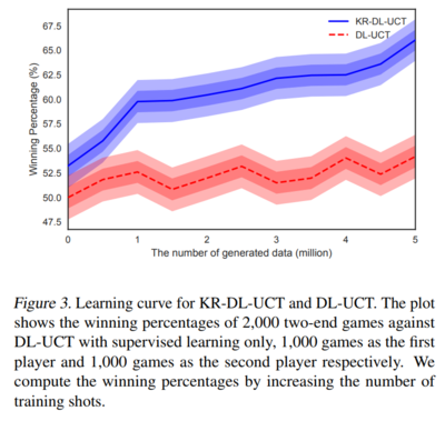
As an evaluation, both algorithms play 2000 games against the DL-UCT algorithm, which is frozen after supervised training. 1000 games are played with the algorithm taking the first, and 100 taking the 2nd, shots. The games were two-end games. The figure below shows each algorithm's winning percentage given different amounts of training data. While the DL-UCT outperforms the supervised-training-only-DL-UCT algorithm, the KR-DL-UCT algorithm performs much better.

Matches

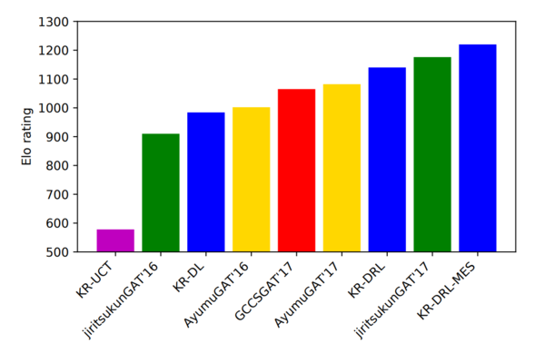
Finally, to test the performance of their multiple algorithms, the authors run matches between their algorithms and other existing programs. Each algorithm plays 200 matches against each other program, 100 of which are played as the first-playing team, and 100 as the second-playing team. Only 1 program was able to out-perform the KR-DRL algorithm. The authors state that this program, JiritsukunGAT'17 also uses a deep network and hand-crafted features. However, the KR-DRL-MES algorithm was still able to out-perform this. Figure 4 shows the Elo ratings of the different programs. Note that the programs in blue are those created by the authors. They also played some games between their KR-DRL-MES and notable programs. Table 1, shows the details of the match results. JiritsukunGAT'17 shows a similar level of performance but KR-DRL-MES is still the winner.

Figure 4. Elo rating and winning percentages of our models and GAT rankers. Each match has 200 games (each program plays 100 pre-ordered games), because the player which has the last shot (the hammer shot) in each end would have an advantage.

Table 1. The 8-end game results for KR-DRL-MES against other programs alternating the opening player each game. The matches are held by following the rules of the latest GAT competition.

Critique

Strengths

This algorithm out-performs other high-performance algorithms (including past competition champions).

I think the paper does a decent job of comparing the performance of their algorithm to others. They are able to clearly show the benefits of many of their additions.

The authors do seem to be able to adopt strategies similar to those used in Go and other games to the continuous action-space domain. In addition, the final strategy needs no hand-crafted features for learning.

Weaknesses

Somtimes, I found this paper difficult to follow. One problem was that the algorithms were introduced first, and then how they were used was described. So when the paper stated that self-play shots were taken after 400 simulations, it seemed unclear what simulations were being run and at what stage of the algorithm (ex: MCTS simulations, simulations sped up by using the value network, full simulations on the curling simulator). In particular, both the MCTS statistics and the policy-value network could be used to estimate both action probabilities and state values, so it is difficult to tell which is used in which case. There was also no clear distinction between discrete-space actions and continuous-space actions.

While I think the comparison of different algorithms was done well, I believe it still lacked some good detail. There were one-off mentions in the paper which would have been nice to see as results. These include the statement that having a policy-value network in place of two networks lead to better performance.

At this point, the algorithms used still rely on initialization by a pre-made program.

There was little theoretical development or justification done in this paper.

While curling is an interesting choice for demonstrating the algorithm, the fact that the simulations used did not support many of the key points of curling (ice conditions, sweeping) seems very limited. Another game, such as pool, would likely have offered some of the same challenges but offered more high-fidelity simulations/training.

While the spatial placements of stones were discretized in a grid, the curl of thrown stones was discretized to only +/-1. This seems like it may limit learning high- and low-spin moves. It should be noted that having zero spins is not commonly used, to the best of my knowledge.

References

1. Lee, K., Kim, S., Choi, J. & Lee, S. "Deep Reinforcement Learning in Continuous Action Spaces: a Case Study in the Game of Simulated Curling." Proceedings of the 35th International Conference on Machine Learning, in PMLR 80:2937-2946 (2018)
2. https://www.baeldung.com/java-monte-carlo-tree-search
3. https://jeffbradberry.com/posts/2015/09/intro-to-monte-carlo-tree-search/
4. https://int8.io/monte-carlo-tree-search-beginners-guide/
5. https://en.wikipedia.org/wiki/Monte_Carlo_tree_search
6. Silver, D., Huang, A., Maddison, C., Guez, A., Sifre, L.,Van Den Driessche, G., Schrittwieser, J., Antonoglou, I.,Panneershelvam, V., Lanctot, M., Dieleman, S., Grewe,D., Nham, J., Kalchbrenner, N.,Sutskever, I., Lillicrap, T.,Leach, M., Kavukcuoglu, K., Graepel, T., and Hassabis,D. Mastering the game of go with deep neural networksand tree search. Nature, pp. 484–489, 2016.
7. Silver, D., Schrittwieser, J., Simonyan, K., Antonoglou,I., Huang, A., Guez, A., Hubert, T., Baker, L., Lai, M., Bolton, A., Chen, Y., Lillicrap, T., Hui, F., Sifre, L.,van den Driessche, G., Graepel, T., and Hassabis, D.Mastering the game of go without human knowledge.Nature, pp. 354–359, 2017.
8. Yamamoto, M., Kato, S., and Iizuka, H. Digital curling strategy based on game tree search. In Proceedings of the IEEE Conference on Computational Intelligence and Games, CIG, pp. 474–480, 2015.
9. Ohto, K. and Tanaka, T. A curling agent based on the montecarlo tree search considering the similarity of the best action among similar states. In Proceedings of Advances in Computer Games, ACG, pp. 151–164, 2017.
10. Ito, T. and Kitasei, Y. Proposal and implementation of digital curling. In Proceedings of the IEEE Conference on Computational Intelligence and Games, CIG, pp. 469–473, 2015.
11. Ioffe, S. and Szegedy, C. Batch normalization: Accelerating deep network training by reducing internal covariate shift. In Proceedings of the International Conference on Machine Learning, ICML, pp. 448–456, 2015.
12. Nair, V. and Hinton, G. Rectified linear units improve restricted boltzmann machines.