CapsuleNets

The paper "Dynamic Routing Between Capsules" was written by three researchers at Google Brain: Sara Sabour, Nicholas Frosst, and Geoffrey E. Hinton. This paper was published and presented at the 31st Conference on Neural Information Processing Systems (NIPS 2017) in Long Beach, California. The same three researchers recently published a highly related paper "Matrix Capsules with EM Routing" for ICLR 2018.

Motivation

Ever since AlexNet eclipsed the performance of competing architectures in the 2012 ImageNet challenge, convolutional neural networks have maintained their dominance in computer vision applications. Despite the recent successes and innovations brought about by convolutional neural networks, some assumptions made in these networks are perhaps unwarranted and deficient. Using a novel neural network architecture, the authors create CapsuleNets, a network that they claim is able to learn image representations in a more robust, human-like manner. With only a 3 layer capsule network, they achieved near state-of-the-art results on MNIST.

Adversarial Examples

First discussed by Christian Szegedy et. al. in late 2013, adversarial examples have been heavily discussed by the deep learning community as a potential security threat to AI learning. Adversarial examples are defined as inputs that an attacker creates intentionally fool a machine learning model. An example of an adversarial example is shown below:

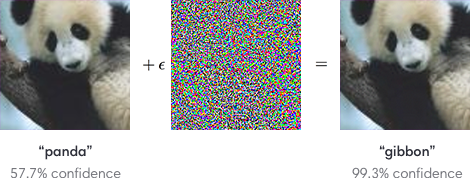
To the human eye, the image appears to be a panda both before and after noise is injected into the image, whereas the trained ConvNet model discerns the noisy image as a Gibbon with almost 100% certainty. The fact that the network is unable to classify the above image as a panda after the epsilon perturbation leads to many potential security risks in AI dependent systems such as self-driving vehicles. Although various methods have been suggested to combat adversarial examples, robust defences are hard to construct due to the inherent difficulties in constructing theoretical models for the adversarial example crafting process. However, beyond the fact that these examples may serve as a security threat, it emphasizes that these convolutional neural networks do not learn image classification/object detection patterns the same way that a human would. Rather than identifying the core features of a panda such as: its eyes, mouth, nose, and the gradient changes in its black/white fur, the convolutional neural network seems to be learning image representations in a completely different manner. Deep learning researchers often attempt to model neural networks after human learning, and it is clear that further steps must be taken to robustify ConvNets against targeted noise perturbations.

Drawbacks of CNNs

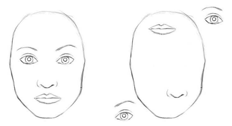
Hinton claims that the key fault with traditional CNNs lies within the pooling function. Although pooling builds translational invariance into the network, it fails to preserve spatial relationships between objects. When we pool, we effectively reduce a kxk kernel of convolved cells into a scalar input. This results in a desired local invariance without inhibiting the network's ability to detect features, but causes valuable spatial information to be lost.

In the example below, the network is able to detect the similar features (eyes, mouth, nose, etc) within both images, but fails to recognize that one image is a human face, while the other is a Picasso-esque due to the CNN's inability to encode spatial relationships after multiple pooling layers.

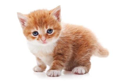
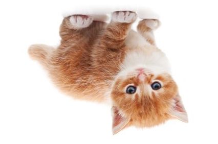
Conversely, we hope that a CNN can recognize that both of the following pictures contain a kitten. Unfortunately, when we feed the two images into a ResNet50 architecture, only the first image is correctly classified, while the second image is predicted to be a guinea pig.

For a more in depth discussion on the problems with ConvNets, please listen to Geoffrey Hinton's talk "What is wrong with convolutional neural nets?" given at MIT during the Brain & Cognitive Sciences - Fall Colloquium Series (December 4, 2014).

Intuition for Capsules

Human vision ignores irrelevant details by using a carefully determined sequence of fixation points to ensure that only a tiny fraction of the optic array is ever processed at the highest resolution. Hinton argues that our brains reason visual information by deconstructing it into a hierarchical representation which we then match to familiar patterns and relationships from memory. The key difference between this understanding and the functionality of CNNs is that recognition of an object should not depend on the angle from which it is viewed.

To enforce rotational and translational equivariance, Capsule Networks store and preserve hierarchical pose relationships between objects. The core idea behind capsule theory is the explicit numerical representations of relative relationships between different objects within an image. Building these relationships into the Capsule Networks model, the network is able to recognize newly seen objects as a rotated view of a previously seen object. For example, the below image shows the Statue of Liberty under five different angles. If a person had only seen the Statue of Liberty from one angle, they would be able to ascertain that all five pictures below contain the same object (just from a different angle).

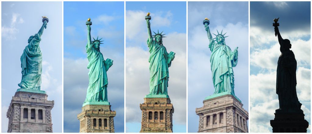
Building on this idea of hierarchical representation of spatial relationships between key entities within an image, the authors introduce Capsule Networks. Unlike traditional CNNs, Capsule Networks are better equipped to classify correctly under rotational invariance. Furthermore, the authors managed to achieve state of the art results on MNIST using a fraction of the training samples that alternative state of the art networks require.

Background, Notation, and Definitions

What is a Capsule

"Each capsule learns to recognize an implicitly defined visual entity over a limited domain of viewing conditions and deformations and it outputs both the probability that the entity is present within its limited domain and a set of “instantiation parameters” that may include the precise pose, lighting and deformation of the visual entity relative to an implicitly defined canonical version of that entity. When the capsule is working properly, the probability of the visual entity being present is locally invariant — it does not change as the entity moves over the manifold of possible appearances within the limited domain covered by the capsule. The instantiation parameters, however, are “equivariant” — as the viewing conditions change and the entity moves over the appearance manifold, the instantiation parameters change by a corresponding amount because they are representing the intrinsic coordinates of the entity on the appearance manifold."

In essence, capsules store object properties in a vector form; probability of detection is encoded as the vector's length, while spatial properties are encoded as the individual vector components. Thus, when a feature is present but the image captures it under a different angle, the probability of detection remains unchanged.

Notation

We want the length of the output vector of a capsule to represent the probability that the entity represented by the capsule is present in the current input. The paper performs a non-linear squashing operation to ensure that vector length falls between 0 and 1, with shorter vectors (less likely to exist entities) being shrunk towards 0.

\begin{align} \mathbf{v}_j &= \frac{||\mathbf{s}_j||^2}{1+ ||\mathbf{s}_j||^2} \frac{\mathbf{s}_j}{||\mathbf{s}_j||^2} \end{align}

where [math]\displaystyle{ \mathbf{v}_j }[/math] is the vector output of capsule [math]\displaystyle{ j }[/math] and [math]\displaystyle{ s_j }[/math] is its total input.

For all but the first layer of capsules, the total input to a capsule [math]\displaystyle{ s_j }[/math] is a weighted sum over all “prediction vectors” [math]\displaystyle{ \hat{\mathbf{u}}_{j|i} }[/math] from the capsules in the layer below and is produced by multiplying the output [math]\displaystyle{ \mathbf{u}i }[/math] of a capsule in the layer below by a weight matrix [math]\displaystyle{ \mathbf{W}ij }[/math]

\begin{align} \mathbf{s}_j = \sum_i c_{ij}\hat{\mathbf{u}}_{j|i}, \hat{\mathbf{u}}_{j|i}= \mathbf{W}_{ij}\mathbf{u}_i \end{align} where the [math]\displaystyle{ c_{ij} }[/math] are coupling coefficients that are determined by the iterative dynamic routing process.

The coupling coefficients between capsule [math]\displaystyle{ i }[/math] and all the capsules in the layer above sum to 1 and are determined by a “routing softmax” whose initial logits [math]\displaystyle{ b_{ij} }[/math] are the log prior probabilities that capsule [math]\displaystyle{ i }[/math] should be coupled to capsule [math]\displaystyle{ j }[/math].

\begin{align} c_{ij} = \frac{\exp(b_{ij})}{\sum_k \exp(b_{ij})} \end{align}

Network Training and Dynamic Routing

Understanding Capsules

The notation can get somewhat confusing, so I will provide intuition behind the computational steps within a capsule. The following image is taken from naturomic's talk on Capsule Networks.

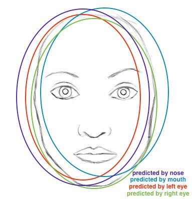
The above image illustrates the key mathematical operations happening within a capsule (and compares them to the structure of a neuron). Although the operations are rather straightforward, it's crucial to note that the capsule computes an affine transformation onto each input vector. The length of the input vectors [math]\displaystyle{ \mathbf{u}_{i} }[/math] represent the probability of entity [math]\displaystyle{ i }[/math] existing in a lower level. This vector is then reoriented with an affine transform using [math]\displaystyle{ \mathbf{W}_{ij} }[/math] matrices that encode spatial relationships between entity [math]\displaystyle{ \mathbf{u}_{i} }[/math] and other lower level features.

We illustrate the intuition behind vector-to-vector matrix multiplication within capsules using the following example: if vectors [math]\displaystyle{ \mathbf{u}_{1} }[/math], [math]\displaystyle{ \mathbf{u}_{2} }[/math], and [math]\displaystyle{ \mathbf{u}_{3} }[/math] represent detection of eyes, nose, and mouth respectively, then after multiplication with trained weight matrices [math]\displaystyle{ \mathbf{W}_{ij} }[/math] (where j denotes existence of a face), we should get a general idea of the general location of the higher level feature (face), similar to the image below.

Dynamic Routing

A capsule [math]\displaystyle{ i }[/math] in a lower-level layer needs to decide how to send its output vector to higher-level capsules [math]\displaystyle{ j }[/math]. This decision is made with probability proportional to [math]\displaystyle{ c_{ij} }[/math]. If there are [math]\displaystyle{ K }[/math] capsules in the level that capsule [math]\displaystyle{ i }[/math] routes to, then we know the following properties about [math]\displaystyle{ c_{ij} }[/math]: [math]\displaystyle{ \sum_{j=1}^M c_{ij} = 1, c_{ij} \geq 0 }[/math]

In essence, the [math]\displaystyle{ \{c_{ij}\}_{j=1}^M }[/math] denotes a discrete probability distribution with respect to capsule [math]\displaystyle{ i }[/math]'s output location. Lower level capsules decide which higher level capsules to send vectors into by adjusting the corresponding routing weights [math]\displaystyle{ \{c_{ij}\}_{j=1}^M }[/math]. After a few iterations in training, numerous vectors will have already been sent to all higher level capsules. Based on the similarity between the current vector being routed and all vectors already sent into the higher level capsules, we decide which capsule to send the current vector into.

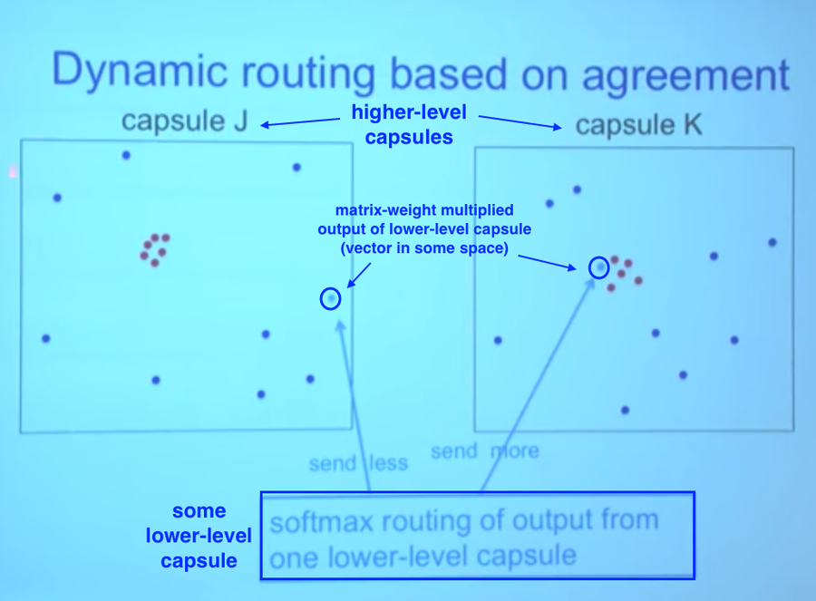
In the image above, we notice that a cluster of points similar to the current vector has already been routed into capsule K, while most points in capsule J are high dissimilar. It thus makes more sense to route the current observation into capsule K; we adjust the corresponding weight upwards during training.

These weights are determined through the dynamic routing procedure:

Although dynamic routing is not the only manner in which we can encode relationships between capsules, the premise of the paper is to demonstrate the capabilities of capsules under a simple implementation. Since the paper's release in 2017, numerous alternative routing implementations have been released including an EM matrix routing algorithm by the same authors (ICLR 208).

Architecture

The capsule network architecture given by the authors has 11.36 million trainable parameters. The paper itself is not very detailed on exact implementation of each architectural layer, and hence it leaves some degree of ambiguity on coding various aspects of the original network. The capsule network has 6 overall layers, with the first three layers denoting components of the encoder, and the last 3 denoting components of the decoder.

Loss Function

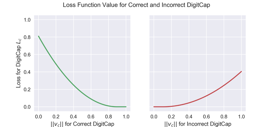
The cost function looks very complicated, but can be broken down into intuitive components. Before diving into the equation, remember that the length of the vector denotes the probability of object existence. The left side of the equation denotes loss when the network classifies an observation correctly; the term becomes zero when classification is incorrect. To compute loss when the network correctly classifies the label, we subtract the vector norm from a fixed quantity [math]\displaystyle{ m^+ := 0.9 }[/math]. On the other hand, when the network classifies a label incorrectly, we penalize the loss based on the network's confidence in the incorrect label; we compute the loss by subtracting [math]\displaystyle{ m^- := 0.1 }[/math] from the vector norm.

A graphical representation of loss function values under varying vector norms is given below.

Encoder Layers

All experiments within this paper were conducted on the MNIST dataset, and thus the architecture is built to classify the corresponding dataset. For more complex datasets, the experiments were less promising.

The encoder layer takes in a 28x28 MNIST image, and learns a 16 dimensional representation of instantiation parameters.

Layer 1: Convolution: This layer is a standard convolution layer. Using kernels with size 9x9x1, a stride of 1, and a ReLU activation function, we detect the 2D features within the network.

Layer 2: PrimaryCaps: We represent the low level features detected during convolution as 32 primary capsules. Each capsule applies eight convolutional kernels with stride 2 to the output of the convolution layer, and feeds the corresponding transformed tensors into the DigiCaps layer.

Layer 3: DigiCaps: This layer contains 10 digit capsules, one for each digit. As explained in the dynamic routing procedure, each input vector from the PrimaryCaps layer has its own corresponding weight matrix [math]\displaystyle{ W_{ij} }[/math]. Using the routing coefficients [math]\displaystyle{ c_{ij} }[/math] and temporary coefficients [math]\displaystyle{ b_{ij} }[/math], we train the DigiCaps layer to output a ten 16 dimensional vectors. The length of the [math]\displaystyle{ i^{th} }[/math] vector in this layer corresponds to the probability of detection of digit [math]\displaystyle{ i }[/math].

Decoder Layers

The decoder layer aims to train the capsules to extract meaningful features for image detection/classification. During training, it takes the 16 layer instantiation vector of the correct (not predicted) DigiCaps layer, and attempts to recreate the 28x28 MNIST image as best as possible. Setting the loss function as reconstruction error (Euclidean distance between reconstructed image and original image), we tune the capsules to encode features that are meaningful within the actual image.

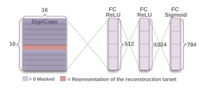
The layer consists of three fully connected layers, and transforms a 16x1 vector from the encoder layer into a 28x28 image.

In addition to the digicaps loss function, we add reconstruction error as a form of regularization. We minimize the Euclidean distance between the outputs of the logistic units and the pixel intensities of the original and reconstructed images. We scale down this reconstruction loss by 0.0005 so that it does not dominate the margin loss during training. As illustrated below, reconstructions from the 16D output of the CapsNet are robust while keeping only important details.

MNIST Experimental Results

Accuracy

The paper tests on the MNIST dataset with 60K training examples, and 10K testing. Wan et al. [2013] achieves 0.21% test error with ensembling and augmenting the data with rotation and scaling. They achieve 0.39% without them. As shown in Table 1, the authors manage to achieve 0.25% test error with only a 3 layer network; the previous state of the art only beat this number with very deep networks. This example shows the importance of routing and reconstruction regularizer, which boosts the performance. On the other hand, while the accuracies are very high, the number of parameters is much smaller compared to the baseline model.

What Capsules Represent for MNIST

The following figure shows the digit representation under capsules. Each row shows the reconstruction when one of the 16 dimensions in the DigitCaps representation is tweaked by intervals of 0.05 in the range [−0.25, 0.25]. By tweaking the values, we notice how the reconstruction changes, and thus get a sense for what each dimension is representing. The authors found that some dimensions represent global properties of the digits, while other represent localized properties.

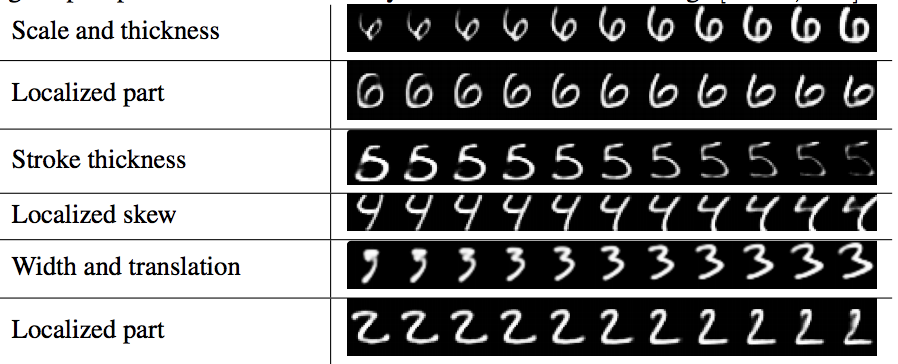
One example the authors provide is: different dimensions are used for the length of the ascender of a 6 and the size of the loop. The variations include stroke thickness, skew and width, as well as digit-specific variations. The authors are able to show dimension representations using a decoder network by feeding a perturbed vector.

Robustness of CapsNet

The authors conclude that DigitCaps capsules learn more robust representations for each digit class than traditional CNNs. The trained CapsNet becomes moderately robust to small affine transformations in the test data.

To compare the robustness of CapsNet to affine transformations against traditional CNNs, both models (CapsNet and a traditional CNN with MaxPooling and DropOut) were trained on a padded and translated MNIST training set, in which each example is an MNIST digit placed randomly on a black background of 40 × 40 pixels. The networks were then tested on the affNIST dataset (MNIST digits with random affine transformation). An under-trained CapsNet which achieved 99.23% accuracy on the MNIST test set achieved a corresponding 79% accuracy on the affnist test set. A traditional CNN achieved similar accuracy (99.22%) on the mnist test set, but only 66% on the affnist test set.

MultiMNIST & Other Experiments

MultiMNIST

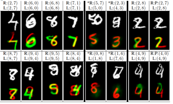
To evaluate the performance of the model on highly overlapping digits, the authors generate a 'MultiMNIST' dataset. In MultiMNIST, images are two overlaid MNIST digits of the same set(train or test) but different classes. The results indicate a classification error rate of 5%. Additionally, CapsNet can be used to segment the image into the two digits that compose it. Moreover, the model is able to deal with the overlaps and reconstruct digits correctly since each digit capsule can learn the style from the votes of PrimaryCapsules layer (Figure 5).

There are some additional steps to generating the MultiMNIST dataset.

1. Both images are shifted by up to 4 pixels in each direction resulting in a 36 × 36 image. Bounding boxes of digits in MNIST overlap by approximately 80%, so this is used to make both digits identifiable (since there is no RGB difference learnable by the network to separate the digits)

2. The label becomes a vector of two numbers, representing the original digit and the randomly generated (and overlaid) digit.

Figure 5: Sample reconstructions of a CapsNet with 3 routing iterations on MultiMNIST test dataset. The two reconstructed digits are overlayed in green and red as the lower image. The upper image shows the input image. L:(l1; l2) represents the label for the two digits in the image and R:(r1; r2) represents the two digits used for reconstruction. The two right most columns show two examples with wrong classification reconstructed from the label and from the prediction (P). In the (2; 8) example the model confuses 8 with a 7 and in (4; 9) it confuses 9 with 0. The other columns have correct classifications and show that the model accounts for all the pixels while being able to assign one pixel to two digits in extremely difficult scenarios (column 1 − 4). Note that in dataset generation the pixel values are clipped at 1. The two columns with the (*) mark show reconstructions from a digit that is neither the label nor the prediction. These columns suggests that the model is not just finding the best fit for all the digits in the image including the ones that do not exist. Therefore in case of (5; 0) it cannot reconstruct a 7 because it knows that there is a 5 and 0 that fit best and account for all the pixels. Also, in case of (8; 1) the loop of 8 has not triggered 0 because it is already accounted for by 8. Therefore it will not assign one pixel to two digits if one of them does not have any other support.

Critique

Although the network performs incredibly favourably in the author's experiments, it has a long way to go on more complex datasets. On CIFAR 10, the network achieved subpar results, and the experimental results seem to worsen the more complex the problem becomes. This is to be expected, since these networks are still in their early stage; later innovations might come in the upcoming decades/years.

Hinton talks about CapsuleNets revolutionizing areas such as self-driving, but such groundbreaking innovations are a long ways away from CIFAR10, and even further from MNIST. Only will time tell if CapsNets will live up to their hype.

Capsules inherently segment images, and learn a lower dimensional embedding in a new manner, which makes them likely to perform well on segmentation and computer vision tasks once further research is done on them.

Additionally these networks are more interpretable than CNNs, and have strong theoretical reasoning for why they could work. Naturally, it would be hard for a new architecture to beat the heavily researched/modified CNNs.

• ([1]) it's not fully clear how effective it can be performed / how scalable it is. Evaluation is performed on a small dataset for shape recognition. The approach will need to be tested on larger, more challenging datasets.

Future Work

The same authors [N. F. Geoffrey E Hinton, Sara Sabour] presented another paper "MATRIX CAPSULES WITH EM ROUTING" in ICLR 2018, which achieved better results than the work presented in this paper. They presented a novel capsule type, where each capsule has a logistic unit and a 4x4 pose matrix. This new type reduced number of errors by 45%, and performed better than standard CNN on white box adversarial attacks. Moreover, we may try to change the curvature and sensitivities to various factors by introducing new form of loss function. It may improve the performance of the model for more complicated data set which is one of the model's drawback.

References

1. N. F. Geoffrey E Hinton, Sara Sabour. Matrix capsules with em routing. In International Conference on Learning Representations, 2018.
2. S. Sabour, N. Frosst, and G. E. Hinton, “Dynamic routing between capsules,” arXiv preprint arXiv:1710.09829v2, 2017
3. Hinton, G. E., Krizhevsky, A. and Wang, S. D. (2011), Transforming Auto-encoders
4. Geoffrey Hinton's talk: What is wrong with convolutional neural nets? - Talk given at MIT. Brain & Cognitive Sciences - Fall Colloquium Series. [2]
5. Understanding Hinton’s Capsule Networks - Max Pechyonkin's series [3]