policy optimization with demonstrations

Introduction

Introduction

The reinforcement learning (RL) method has made significant progress in a variety of applications, but the exploration problems that how to gain more experience from novel policy to improve long-term performance are still challenges, especially in environments where reward signals are sparse and rare. There are currently two ways to solve such exploration problems in RL: 1) Guide the agent to explore the state that has never been seen. 2) Guide the agent to imitate the demonstration trajectory sampled from an expert policy to learn. When guiding the agent to imitate the expert behavior for learning, there are also two methods: putting the demonstration directly into the replay memory or using the demonstration trajectory to pre-train the policy in a supervised manner. However, neither of these methods takes full advantage of the demonstration data. To address this problem, a novel policy optimization method based on demonstration (POfD) is proposed, which takes full advantage of the demonstration and there is no need to ensure that the expert policy is the optimal policy. In this paper, the authors evaluate the performance of POfD on Mujoco in sparse-reward environments. The experiments results show that the performance of POfD is greatly improved compared with some strong baselines and it is even compared to the policy gradient method in dense-reward environments.

Intuition

The agent should imitate the demonstrated behavior when rewards are sparse and then explore new states on its own after acquiring sufficient skills, which is a dynamic intrinsic reward mechanism that can be reshaped the native rewards in RL.

Related Work

There are some relates works in overcoming exploration difficulties by learning from demonstration and imitation learning in RL.

For Learning from demonstration (LfD),

1. Most LfD methods adopt value-based RL algorithms, such as DQfD that is applied into the discrete action spaces and DDPGfD that is extends to the continuous spaces. But both of them underutilize the demonstration data.
2. There are some methods based on policy iteration, which shapes the value function by using demonstration data. But they get the bad performance when demonstration data is imperfect.
3. A hybrid framework that learns the policy in which the probability of taking demonstrated actions is maximized is proposed, which considers less demonstration data.
4. A reward reshaping mechanism that encourages taking actions close to the demonstrated ones is proposed. It is similar with the method in this paper, but there is the difference that it is defined a potential function based on multi-variate Gaussian to model the distribution of state-actions.

All of the above methods require a lot of perfect demonstration data to get satisfactory performance, which is different from POfD in this paper.

For imitation learning,

1. Inverse Reinforce Learning problems are solved by alternating between fitting the reward function and selecting the policy. But it cannot be extended to big-scale problems.
2. Generative Adversarial Imitation Learning (GAIL) uses a discriminator to distinguish whether a state-action pair is from the expert or the learned policy and it can be applied into the high-dimensional continuous control problems.

All of the above methods are effective for imitation learning, but they usually suffer the bad performance when the expert data is imperfect. That is different from POfD in this paper.

Background

Preliminaries

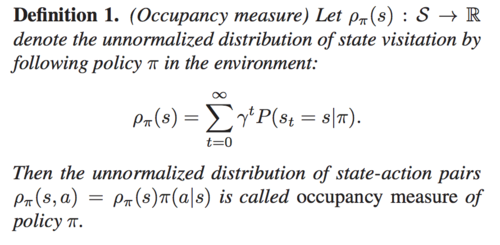
Markov Decision Process (MDP) is defined by a tuple [math]\displaystyle{ ⟨S, A, P, r, \gamma⟩ }[/math], where [math]\displaystyle{ S }[/math] is the state, [math]\displaystyle{ A }[/math]is the action, [math]\displaystyle{ P(s'|s,a) }[/math] is the transition distribution of taking action [math]\displaystyle{ a }[/math] at state [math]\displaystyle{ s }[/math], [math]\displaystyle{ r(s,a) }[/math]is the reward function, and [math]\displaystyle{ \gamma }[/math] is discounted factor between 0 and 1. Policy [math]\displaystyle{ \pi(a|s) }[/math] is a mapping from states to action, the performance of [math]\displaystyle{ \pi }[/math] is usually evaluated by its expected discounted reward [math]\displaystyle{ \eta(\pi) }[/math]: \[\eta(\pi)=\mathbb{E}_{\pi}[r(s,a)]=\mathbb{E}_{(s_0,a_0,s_1,...)}[\sum_{t=0}^\infty\gamma^{t}r(s_t,a_t)] \] The value function is [math]\displaystyle{ V_{\pi}(s) =\mathbb{E}_{\pi}[r(·,·)|s_0=s] }[/math], the action value function is [math]\displaystyle{ Q_{\pi}(s,a) =\mathbb{E}_{\pi}[r(·,·)|s_0=s,a_0=a] }[/math], and the advantage function that reflects the expected additional reward after taking action a at state s is [math]\displaystyle{ A_{\pi}(s,a)=Q_{\pi}(s,a)-V_{\pi}(s) }[/math]. Then the authors define Occupancy measure, which is used to estimate the probability that state [math]\displaystyle{ s }[/math] and state action pairs [math]\displaystyle{ (s,a) }[/math] when executing a certain policy.

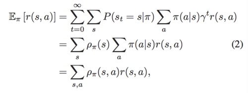
Then the performance of [math]\displaystyle{ \pi }[/math] can be rewritten to:

At the same time, the authors propose a lemma:

Problem Definition

In this paper, the authors aim to develop a method that can boost exploration by leveraging effectively the demonstrations [math]\displaystyle{ D^E }[/math]from the expert policy [math]\displaystyle{ \pi_E }[/math] and maximize [math]\displaystyle{ \eta(\pi) }[/math] in the sparse-reward environment. The authors define the demonstrations [math]\displaystyle{ D^E=\{\tau_1,\tau_2,...,\tau_N\} }[/math], where [math]\displaystyle{ \tau_i=\{(s_0^i,a_0^i),(s_1^i,a_1^i),...,(s_T^i,a_T^i)\} }[/math] is generated from the expert policy. In addition, there is an assumption on the quality of the expert policy:

Moreover, it is not necessary to ensure that the expert policy is advantageous over all the policies. It is because that POfD will learn a better policy than expert policy by exploring on its own in later learning stages.

Method

Policy Optimization with Demonstration (POfD)

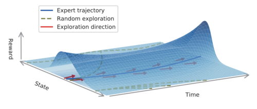
This method optimizes the policy by forcing the policy to explore in the nearby region of the expert policy that is specified by several demonstrated trajectories [math]\displaystyle{ D^E }[/math] (as shown in Fig.1) in order to avoid causing slow convergence or failure when the environment feedback is sparse. In addition, the authors encourage the policy π to explore by "following" the demonstrations DE. Thus, a new learning objective is given: \[ \mathcal{L}(\pi_{\theta})=-\eta(\pi_{\theta})+\lambda_{1}D_{JS}(\pi_{\theta},\pi_{E})\] where [math]\displaystyle{ D_{JS}(\pi_{\theta},\pi_{E}) }[/math] is Jensen-Shannon divergence between current policy [math]\displaystyle{ \pi_{\theta} }[/math] and the expert policy [math]\displaystyle{ \pi_{E} }[/math] , [math]\displaystyle{ \lambda_1 }[/math] is a trading-off parameter, and [math]\displaystyle{ \theta }[/math] is policy parameter. According to Lemma 1, the authors use [math]\displaystyle{ D_{JS}(\rho_{\theta},\rho_{E}) }[/math] to instead of [math]\displaystyle{ D_{JS}(\pi_{\theta},\pi_{E}) }[/math], because it is easier to optimize through adversarial training on demonstrations. The learning objective is: \[ \mathcal{L}(\pi_{\theta})=-\eta(\pi_{\theta})+\lambda_{1}D_{JS}(\rho_{\theta},\rho_{E})\]

Benefits of Exploration with Demonstrations

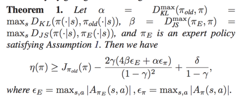
The authors introduce the benefits of POfD. Firstly, we consider the expression of expected return in policy gradient methods. \[ \eta(\pi)=\eta(\pi_{old})+\mathbb{E}_{\tau\sim\pi}[\sum_{t=0}^\infty\gamma^{t}A_{\pi_{old}}(s_t,a_t)]\] [math]\displaystyle{ \eta(\pi) }[/math]is the advantage over the policy πold in the previous iteration, so the expression can be rewritten by \[ \eta(\pi)=\eta(\pi_{old})+\sum_{s}\rho_{\pi}(s)\sum_{a}\pi(a|s)A_{\pi_{old}}(s,a)\] The local approximation to [math]\displaystyle{ \eta(\pi) }[/math] up to first order is usually as the surrogate learning objective to be optimized by policy gradient methods due to the difficulties brought by complex dependency of [math]\displaystyle{ \rho_{\pi}(s) }[/math] over [math]\displaystyle{ \pi }[/math]: \[ J_{\pi_{old}}(\pi)=\eta(\pi_{old})+\sum_{s}\rho_{\pi_{old}}(s)\sum_{a}\pi(a|s)A_{\pi_{old}}(s,a)\] The policy gradient methods improve [math]\displaystyle{ \eta(\pi) }[/math] monotonically by optimizing the above [math]\displaystyle{ J_{\pi_{old}}(\pi) }[/math] with a sufficiently small update step from [math]\displaystyle{ \pi_{old} }[/math] to [math]\displaystyle{ \pi }[/math] such that [math]\displaystyle{ D_{KL}^{max}(\pi, \pi_{old}) }[/math] is bounded. For POfD, it imposes a regularization [math]\displaystyle{ D_{JS}(\pi_{\theta}, \pi_{E}) }[/math] in order to encourage explorations around regions demonstrated by the expert policy. Theorem 1 shows such benefits,

Optimization

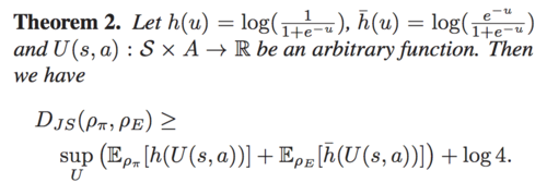
For POfD, the authors choose to optimize the lower bound of learning objective rather than optimizing objective. This optimization method is compatible with any policy gradient methods. Theorem 2 gives the lower bound of [math]\displaystyle{ D_{JS}(\rho_{\theta}, \rho_{E}) }[/math]：

Thus, the lower bound of learning objective is:

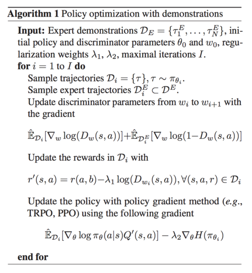
where [math]\displaystyle{ D(s,a)=\frac{1}{1+e^{-U(s,a)}}: S\times A \rightarrow (0,1) }[/math], and its supremum ranging is like a discriminator for distinguishing whether the state-action pair is a current policy or an expert policy. To avoid overfitting, the authors add causal entropy [math]\displaystyle{ −H (\pi_{\theta}) }[/math]as the regularization term. Thus, the learning objective is: \[\min_{\theta}\mathcal{L}=-\eta(\pi_{\theta})-\lambda_{2}H(\pi_{\theta})+\lambda_{1} \sup_{{D\in(0,1)}^{S\times A}} \mathbb{E}_{\pi_{\theta}}[\log(D(s,a))]+\mathbb{E}_{\pi_{E}}[\log(1-D(s,a))]\] At this point, the problem has been like Generative Adversarial Networks (GANs). The difference is that the discriminative model D of GANs is well-trained but the expert policy of POfD is not optimal. Then suppose D is parameterized by w. If it is from an expert policy, [math]\displaystyle{ D_w }[/math]is toward 1, otherwise it is toward 0. Thus, the minimax learning objective is: \[\min_{\theta}\max_{w}\mathcal{L}=-\eta(\pi_{\theta})-\lambda_{2}H (\pi_{\theta})+\lambda_{1}( \mathbb{E}_{\pi_{\theta}}[\log(D_{w}(s,a))]+\mathbb{E}_{\pi_{E}}[\log(1-D_{w}(s,a))])\] The minimax learning objective can be rewritten by substituting the expression of [math]\displaystyle{ \eta(\pi) }[/math]: \[\min_{\theta}\max_{w}-\mathbb{E}_{\pi_{\theta}}[r'(s,a)]-\lambda_{2}H (\pi_{\theta})+\lambda_{1}\mathbb{E}_{\pi_{E}}[\log(1-D_{w}(s,a))]\] where [math]\displaystyle{ r'(s,a)=r(a,b)-\lambda_{1}\log(D_{w}(s,a)) }[/math] is the reshaped reward function. The above objective can be optimized efficiently by alternately updating policy parameters θ and discriminator parameters w, then the gradient is given by: \[\mathbb{E}_{\pi}[\nabla_{w}\log(D_{w}(s,a))]+\mathbb{E}_{\pi_{E}}[\nabla_{w}\log(1-D_{w}(s,a))]\] Then, fixing the discriminator [math]\displaystyle{ D_w }[/math], the reshaped policy gradient is: \[\nabla_{\theta}\mathbb{E}_{\pi_{\theta}}[r'(s,a)]=\mathbb{E}_{\pi_{\theta}}[\nabla_{\theta}\log\pi_{\theta}(a|s)Q'(s,a)]\] where [math]\displaystyle{ Q'(\bar{s},\bar{a})=\mathbb{E}_{\pi_{\theta}}[r'(s,a)|s_0=\bar{s},a_0=\bar{a}] }[/math]. At the end, Algorithm 1 gives the detailed process.

Discussion on Existing LfD Methods

DQFD

DQFD puts the demonstrations into a replay memory D and keeps them throughout the Q-learning process. The objective for DQFD is: \[J_{DQfD}={\hat{\mathbb{E}}}_{D}[(R_t(n)-Q_w(s_t,a_t))^2]+\alpha{\hat{\mathbb{E}}}_{D^E}[(R_t(n)-Q_w(s_t,a_t))^2]\] The second term can be rewritten as [math]\displaystyle{ {\hat{\mathbb{E}}}_{D^E}[(R_t(n)-Q_w(s_t,a_t))^2]={\hat{\mathbb{E}}}_{D^E}[(\hat{\rho}_E(s,a)-\rho_{\pi}(s,a))^{2}r^2(s,a)] }[/math], which can be regarded as a regularization forcing current policy's occupancy measure to match the expert's empirical occupancy measure, weighted by the potential reward.

DDPGfD

DDPGfD also puts the demonstrations into a replay memory D, but it is based on an actor-critic framework. The objective for DDPGfD is the same as DQFD. Its policy gradient is: \[\nabla_{\theta}J_{DDPGfD}\approx \mathbb{E}_{s,a}[\nabla_{a}Q_w(s,a)\nabla_{\theta}\pi_{\theta}(s)], a=\pi_{\theta}(s) \] From this equation, policy is updated relying on learned Q-network [math]\displaystyle{ Q_w }[/math]rather than the demonstrations [math]\displaystyle{ D^{E} }[/math]. DDPGfD shares the same objective function for [math]\displaystyle{ Q_w }[/math] as DQfD, thus they have the same way of leveraging demonstrations, that is the demonstrations in DQfD and DDPGfD induce an occupancy measure matching regularization.

Experiments

Goal

The authors aim at investigating 1) whether POfD can aid exploration by leveraging a few demonstrations, even though the demonstrations are imperfect. 2) whether POfD can succeed and achieve high empirical return, especially in environments where reward signals are sparse and rare.

Settings

The authors conduct the experiments on 8 physical control tasks, ranging from low-dimensional spaces to high-dimensional spaces and naturally sparse environments based on OpenAI Gym and Mujoco. Due to the uniqueness of the environments, the authors introduce 4 ways to sparsity their built-in dense rewards. TYPE1: a reward of +1 is given when the agent reaches the terminal state, and otherwisely 0. TYPE2: a reward of +1 is given when the agent survives for a while. TYPE3: a reward of +1 is given for every time the agent moves forward over a specific number of units in Mujoco environments. TYPE4: specially designed for InvertedDoublePendulum, a reward +1 is given when the second pole stays above a specific height of 0.89. The details are shown in Table 1. Moreover, only one single imperfect trajectory is used as the demonstrations in this paper. The authors collect the demonstrations by training an agent insufficiently by running TRPO in the corresponding dense environment.

Baselines

The authors compare POfD against 5 strong baselines:

• training the policy with TRPO in dense environments, which is called expert
• training the policy with TRPO in sparse environments
• applying GAIL to learn the policy from demonstrations
• DQfD
• DDPGfD

Results

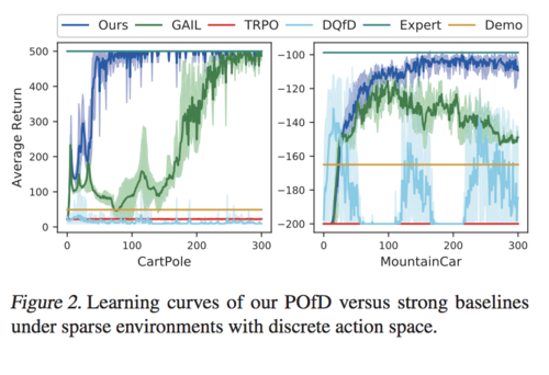
Firstly, the authors test the performance of POfD in sparse control environments with discrete actions. From Table 1, POfD achieves performance comparable with the policy learned under dense environments. From Figure 2, only POfD successes to explore sufficiently and achieves great performance in both sparse environments. TRPO and DQFD fail to explore and GAIL converes to the imperfect demonstration in MountainCar.

Then, the authors test the performance of POfD under spares environments with continuous actions space. From Figure 3, POfD achieves expert-level performance in terms of cumulated rewards.

Conclusion

A method that can acquire knowledge from few and imperfect demonstration data to aid exploration in environments with sparse feedback is proposed, that is POfD. It is compatible with any policy gradient methods. POfD induces implicit dynamic reward shaping and brings provable benefits for policy improvement. Moreover, the experiments results have shown the effectivity of POfD in encouraging the agent to explore around the nearby region of the expert policy and learning better policies.

Critique

1. A novel demonstration-based policy optimization method is proposed. In the process of policy optimization, POfD reshapes the reward function. This new reward function can guide the agent to imitate the expert behavior when the reward is sparse and explore on its own when the reward value can be obtained, which can take full advantage of the demonstration data and there is no need to ensure that the expert policy is the optimal policy.
2. POfD can be combined with any policy gradient methods. Its performance surpasses five strong baselines and can be comparable to the agents that trained in the dense-reward environment.
3. The paper is structured and the flow of ideas is easy to follow. For related work, the authors clearly explain similarities and differences among these related works.
4. This paper's scalability is demonstrated. The experiments environments are ranging from low-dimensional spaces to high-dimensional spaces and from discrete action spaces to continuous actions spaces. For future work, can it be realized in the real world?
5. There is a doubt that whether it is a correct method to use the trajectory that was insufficiently learned in dense-reward environment as the imperfect demonstration.
6. In this paper, the performance only is judged by the cumulative reward, can other evaluation terms be considered? For example, the convergence rate.