Reinforcement Learning of Theorem Proving

Introduction

Automated reasoning over mathematical proof was a major motivation for the development of computer science. Automated theorem provers (ATP) can in principle be used to attack any formally stated mathematical problem and is a research area that has been present since the early 20th century [1]. As of today, state-of-art ATP systems rely on the fast implementation of complete proof calculi. such as resolution and tableau. However, they are still far weaker than trained mathematicians. Within current ATP systems, many heuristics are essential for their performance. As a result, in recent years machine learning has been used to replace such heuristics and improve the performance of ATPs.

In this paper, the authors propose a reinforcement learning based ATP, rlCoP. The proposed ATP reasons within first-order logic. The underlying proof calculi are the connection calculi [2], and the reinforcement learning method is Monte Carlo tree search along with policy and value learning. It is shown that reinforcement learning results in a 42.1% performance increase compared to the base prover (without learning).

Related Work

C. Kalizyk and J. Urban proposed a supervised learning based ATP, FEMaLeCoP, whose underlying proof calculi is the same as this paper in 2015 [3]. Their algorithm learns from existing proofs to choose the next tableau extension step. Since the MaLARea [8] system, number of iterations of a feedback loop between proving and learning have been explored, remarkably improving over human-designed heuristics when reasoning in large theories. However, such systems are known to only learn a high-level selection of relevant facts from a large knowledge base and delegate the internal proof search to standard ATP systems. S. Loos, et al. developed an supervised learning ATP system in 2017 [4], with superposition as their proof calculi. However, they chose deep neural network (CNNs and RNNs) as feature extractor. These systems are treated as black boxes in literature with not much understanding of their performances possible.

In leanCoP [9], one of the simpler connection tableau systems, the next tableau extension step could be selected using supervised learning. In addition, the first experiments with Monte-Carlo guided proof search [5] have been done for connection tableau systems. The improvement over the baseline measured in that work is much less significant than here. This is closest to the authors' approach but the performance is poorer than this paper.

On a different note, A. Alemi, et al. proposed a deep sequence model for premise selection in 2016 [6], and they claim to be the first team to involve deep neural networks in ATPs. Although premise selection is not directly linked to automated reasoning, it is still an important component in ATPs, and their paper provides some insights into how to process datasets of formally stated mathematical problems.

First Order Logic and Connection Calculi

Here we assume basic first-order logic and theorem proving terminology, and we will offer a brief introduction of the bare prover and connection calculi. Let us try to prove the following first-order sentence.

This sentence can be transformed into a formula in Skolemized Disjunctive Normal Form (DNF), which is referred to as the "matrix".

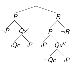
The original first-order sentence is valid if and only if the Skolemized DNF formula is a tautology. The connection calculi attempt to show that the Skolemized DNF formula is a tautology by constructing a tableau. We will start at the special node, root, which is an open leaf. At each step, we select a clause (for example, clause [math]\displaystyle{ P \wedge R }[/math] is selected in the first step), and add the literals as children for an existing open leaf. For every open leaf, examine the path from the root to this leaf. If two literals on this path are unifiable (for example, [math]\displaystyle{ Qx' }[/math] is unifiable with [math]\displaystyle{ \neg Qc }[/math]), this leaf is then closed. An example of a closed tableaux is shown in Figure 1. In standard terminology, it states that a connection is found on this branch.

Figure 1. An example of closed tableaux. Adapted from [2]

The paper's goal is to close every leaf, i.e. on every branch, there exists a connection. If such state is reached, the paper has shown that the Skolemized DNF formula is a tautology, thus proving the original first-order sentence. As we can see from the constructed tableaux, the example sentence is indeed valid.

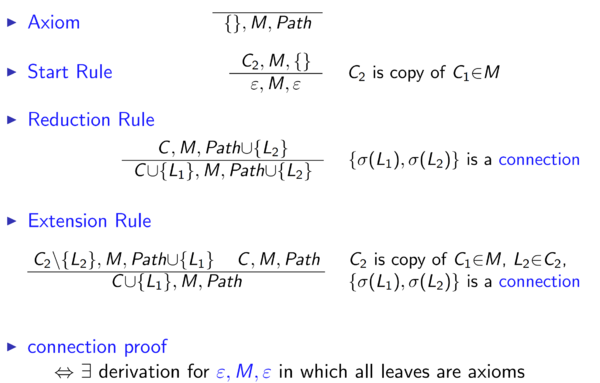
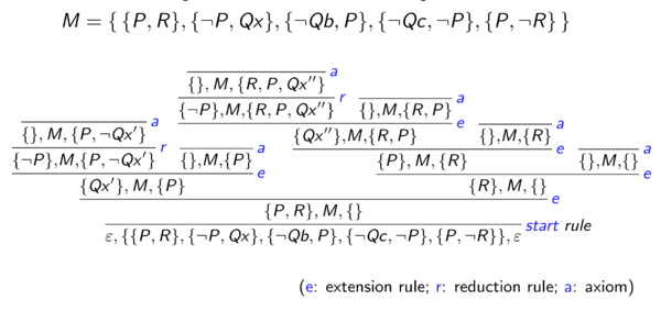
In formal terms, the rules of connection calculi is shown in Figure 2, and the formal tableaux for the example sentence is shown in Figure 3. Each leaf is denoted as [math]\displaystyle{ subgoal, M, path }[/math] where [math]\displaystyle{ subgoal }[/math] is a list of literals that we need to find connection later, [math]\displaystyle{ M }[/math] stands for the matrix, and [math]\displaystyle{ path }[/math] stands for the path leading to this leaf.

Figure 2. Formal connection calculi. Adapted from [2].

Figure 3. Formal tableaux constructed from the example sentence. Adapted from [2].

To sum up, the bare prover follows a very simple algorithm. given a matrix, a non-negated clause is chosen as the first subgoal. The function prove(subgoal, M, path) is stated as follows:

• If subgoal is empty
  • return TRUE
• If reduction is possible
  • Perform reduction, generating new_subgoal, new_path
  • return prove(new_subgoal, M, new_path)
• For all clauses in M
  • If a clause can do extension with subgoal
  • Perform extension, generating new_subgoal1, new_path, new_subgoal2
  • return prove(new_subgoal1, M, new_path) and prove(new_subgoal2, M, path)
• return FALSE

It is important to note that the bare prover implemented in this paper is incomplete. Here is a pathological example. Suppose the following matrix (which is trivially a tautology) is feed into the bare prover. Let clause [math]\displaystyle{ P(0) }[/math] be the first subgoal. Clearly choosing [math]\displaystyle{ \neg P(0) }[/math] to extend will complete the proof.

However, if we choose [math]\displaystyle{ \neg P(x) \lor P(s(x)) }[/math] to do extension, the algorithm will generate an infinite branch [math]\displaystyle{ P(0), P(s(0)), P(s(s(0))) ... }[/math]. It is the task of reinforcement learning to guide the prover in such scenarios towards a successful proof.

In addition, the provability of first-order sentences is generally undecidable (this result is named the Church-Turing Thesis), which sheds light on the difficulty of automated theorem proving.

Mizar Math Library

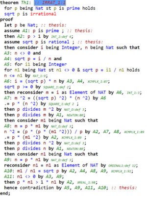
Mizar Math Library (MML) is a library of mathematical theories. The axioms behind the library is the Tarski-Grothendieck set theory, written in first-order logic. The library contains 57,000+ theorems and their proofs, along with many other lemmas, as well as unproven conjectures. Figure 4 shows a Mizar article of the theorem "If [math]\displaystyle{ p }[/math] is prime, then [math]\displaystyle{ \sqrt p }[/math] is irrational."

Figure 4. An article from MML. Adapted from [6].

The training and testing data for this paper is a subset of MML, the Mizar40, which is 32,524 theorems proved by automated theorem provers. Below is an example from the Mizar40 library, it states that with d3_xboole_0 and t3_xboole_0 as premises, we can prove t5_xboole_0.

Monte Carlo Guidance

Monte Carlo tree search (MCTS) is a heuristic search algorithm for some kinds of decision processes. The focus of Monte Carlo tree search is on the analysis of the most promising moves, expanding the search tree based on random sampling of the search space. Then the expansion will then be used to weight the node in the search tree.

In the reinforcement learning setting, the action is defined as one inference (either reduction or extension). The proof state is defined as the whole tableaux. To implement Monte-Carlo tree search, each proof state [math]\displaystyle{ i }[/math] needs to maintain three parameters, its prior probability [math]\displaystyle{ p_i }[/math], its total reward [math]\displaystyle{ w_i }[/math], and number of its visits [math]\displaystyle{ n_i }[/math]. If no policy learning is used, the prior probabilities are all equal to one.

A simple heuristic is used to estimate the future reward of leaf states: suppose leaf state [math]\displaystyle{ i }[/math] has [math]\displaystyle{ G_i }[/math] open subgoals, the reward is computed as [math]\displaystyle{ 0.95 ^ {G_i} }[/math]. This will be replaced once value learning is implemented.

The standard UCT formula is chosen to select the next actions in the playouts \begin{align} {\frac{w_i}{n_i}} + 2 \cdot p_i \cdot {\sqrt{\frac{\log N}{n_i}}} \end{align} where [math]\displaystyle{ N }[/math] stands for the total number of visits of the parent node.

The bare prover is asked to play [math]\displaystyle{ b }[/math] playouts of length [math]\displaystyle{ d }[/math] from the empty tableaux, each playout backpropagates the values of proof states it visits. After these [math]\displaystyle{ b }[/math] playouts a special action (inference) is made, corresponding to an actual move, resulting in a new bigstep tableaux. The next [math]\displaystyle{ b }[/math] playouts will start from this tableaux, followed by another bigstep, etc.

Policy Learning and Guidance

From many runs of MCT, we will know the prior probability of actions (inferences) in particular proof states, we can extract the frequency of each action [math]\displaystyle{ a }[/math], and normalize it by dividing with the average action frequency at that state, resulting in a relative proportion [math]\displaystyle{ r_a \in (0, \infty) }[/math]. We characterize the proof states for policy learning by extracting human-engineered features. Also, we characterize actions by extracting features from the clause chosen and literal chosen as well. Thus we will have a feature vector [math]\displaystyle{ (f_s, f_a) }[/math].

The feature vector [math]\displaystyle{ (f_s, f_a) }[/math] is regressed against the associated [math]\displaystyle{ r_a }[/math].

During the proof search, the prior probabilities [math]\displaystyle{ p_i }[/math] of available actions [math]\displaystyle{ a_i }[/math] in a state [math]\displaystyle{ s }[/math] is computed as the softmax of their predictions.

Training examples are only extracted from big step states, making the amount of training data manageable.

Value Learning and Guidance

Bigstep states are also used for proof state evaluation. For a proof state [math]\displaystyle{ s }[/math], if it corresponds to a successful proof, the value is assigned as [math]\displaystyle{ v_s = 1 }[/math]. If it corresponds to a failed proof, the value is assigned as [math]\displaystyle{ v_s = 0 }[/math]. For other scenarios, denote the distance between state [math]\displaystyle{ s }[/math] and a successful state as [math]\displaystyle{ d_s }[/math], then the value is assigned as [math]\displaystyle{ v_s = 0.99^{d_s} }[/math]

Proof state feature [math]\displaystyle{ f_s }[/math] is regressed against the value [math]\displaystyle{ v_s }[/math]. During the proof search, the reward of leaf states are computed from this prediction.

Features and Learners

For proof states, features are collected from the whole tableaux (subgoals, matrix, and paths). Each unique symbol is represented by an integer, and the tableaux can be represented as a sequence of integers. Term walk is implemented to combine a sequence of integers into a single integer by multiplying components by a fixed large prime and adding them up. Then the resulting integer is reduced to a smaller feature space by taking modulo by a large prime.

For actions the feature extraction process is similar, but the term walk is over the chosen literal and the chosen clause.

In addition to the term walks, they also added several common features: number of goals, total symbol size of all goals, length of active paths, number of current variable instantiations, most common symbols.

The whole project is implemented in OCaml, and XGBoost is ported into OCaml as the learner.

Experimental Results

The authors use the M2k dataset to compare the performance of mlCoP, the bare prover and rlCoP using only UCT.

• Performance without Learning

Table 3 shows the baseline result. The Performance of the bare prover is significantly lower than mlCoP and rlCoP without policy/value.

• Reinforcement Learning of Policy Only

In this experiment, the authors evaluated on the dataset rlCoP with UCT using policy learning only. They used the policy training data from previous iterations to train a new predictor after each iteration. Which means only the first iteration ran without policy while all the rest iterations used previous policy training data. From Table 4, rlCoP is better than mlCoP run with the much higher [math]\displaystyle{ 4 ∗ 10^{6} }[/math] inference limit after fourth iteration.

• Reinforcement Learning of Value Only

This experiment was similar to the last one, however, they used only values rather than learned policy. From Table 5, the performance of rlCoP is close to mlCoP but below it after 20 iterations, and it is far below rlCoP using only policy learning.

• Reinforcement Learning of Policy and Value

From Table 6, the performance of rlCoP is 19.4% more than mlCoP with [math]\displaystyle{ 4 ∗ 10^{6} }[/math] inferences, 13.6% more than the best iteration of rlCoP with policy only, and 44.3% more than the best iteration of rlCoP with value only after 20 iterations.

Besides, they also evaluated the effect of the joint reinforcement learning of both policy and value. Replacing final policy and value with the best one from policy-only or value-only both decreased performance.

• Evaluation on the Whole Miz40 Dataset.

The authors split Mizar40 dataset into 90% training examples and 10% testing examples. 200,000 inferences are allowed for each problem. 10 iterations of policy and value learning are performed (based on MCT). The training and testing results are shown as follows. In the table, mlCoP represents for the bare prover with iterative deepening (i.e. a complete automated theorem prover with connection calculi), and bare prover stands for the prover implemented in this paper, without MCT guidance.

[[file:atp_result0.jpg|frane|550px|center]Figure 5a. Experimental result on Mizar40 dataset]

Figure 5b. More experimental result on Mizar40 dataset

As shown by these results, reinforcement learning leads to a significant performance increase for automated theorem proving, the 42.1% performance improvement is unusually high, since the published improvement in this field is typically between 3% and 10%. [1]

Besides these results, there were also found that some test problems could be solved with rlCoP easily but mlCoP could not.

Conclusions

In this work, the authors developed an automated theorem prover that uses no domain engineering and instead replies on MCT guided by reinforcement learning. The resulting system is more than 40% stronger than the baseline system. The authors believe that this is a landmark in the field of automated reasoning, demonstrating that building general problem solvers by reinforcement learning is a viable approach. [1]

The authors pose that some future research could include strong learning algorithms to characterize mathematical data. The development of suitable deep learning architectures will help the algorithm characterize semantic and syntactic features of mathematical objects which will be crucial to create strong assistants for mathematics and hard sciences.

Critiques

Until now, automated reasoning is relatively new to the field of machine learning, and this paper shows a lot of promise in this research area.

The feature extraction part of this paper is less than optimal. It is my opinion that with proper neural network architecture, deep learning extracted features will be superior to human-engineered features, which is also shown in [4, 6].

Also, the policy-value learning iteration is quite inefficient. The learning loop is:

• Loop
  • Run MCT with the previous model on an entire dataset
  • Collect MCT data
  • Train a new model

If we adopt this to an online learning scheme by learning as soon as MCT generates new data, and update the model immediately, there might be some performance increase.

The experimental design of this paper has some flaws. The authors compare the performance of mlCoP and rlCoP by limiting them to the same number of inference steps. However, every inference step of rlCoP requires additional machine learning prediction, which costs more time. A better way to compare their performance is to set a time limit.

It would also be interesting to study automated theorem proving in another logic system, like high order logic.

References

[1] C. Kaliszyk, et al. Reinforcement Learning of Theorem Proving. NIPS 2018.

[2] J. Otten and W. Bibel. leanCoP: Lean Connection-Based Theorem Proving. Journal of Symbolic Computation, vol. 36, pp. 139-161, 2003.

[3] C. Kaliszyk and J. Urban. FEMaLeCoP: Fairly Efficient Machine Learning Connection Prover. Lecture Notes in Computer Science. vol. 9450. pp. 88-96, 2015.

[4] S. Loos, et al. Deep Network Guided Proof Search. LPAR-21, 2017.

[5] M. F¨arber, C. Kaliszyk, and J. Urban. Monte Carlo tableau proof search. In L. de Moura, editor, 26th International Conference on Automated Deduction (CADE), volume 10395 of LNCS, pages 563–579. Springer, 2017.

[6] A. Alemi, et al. DeepMath-Deep Sequence Models for Premise Selection. NIPS 2016.

[7] Mizar Math Library. http://mizar.org/library/

[8] J. Urban, G. Sutcliffe, P. Pudla ́k, and J. Vyskocˇil. MaLARea SG1 - Machine Learner for Automated Reasoning with Semantic Guidance. In A. Armando, P. Baumgartner, and G. Dowek, editors, IJCAR, volume 5195 of LNCS, pages 441–456. Springer, 2008.

[9] J. Otten and W. Bibel. leanCoP: lean connection-based theorem proving. J. Symb. Comput., 36(1-2):139–161, 2003.