stat441F18/TCNLM

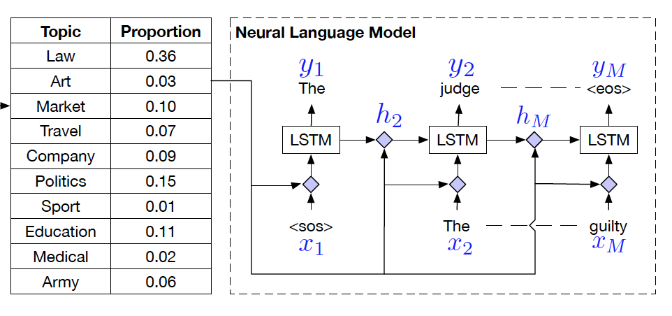
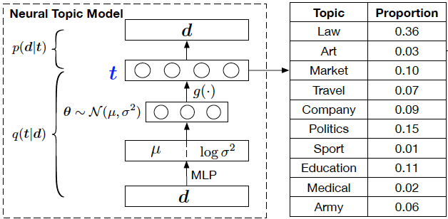
Topic Compositional Neural Language Model (TCNLM) simultaneously captures both the global semantic meaning and the local word-ordering structure in a document. A common TCNLM incorporates fundamental components of both a neural topic model (NTM) and a Mixture-of-Experts (MoE) language model. The latent topics learned within a variational autoencoder framework, coupled with the probability of topic usage, are further trained in a MoE model. (Insert figure here)

TCNLM networks are well-suited for topic classification and sentence generation on a given topic. The combination of latent topics, weighted by the topic-usage probabilities, yields an effective prediction for the sentences. TCNLMs were also developed to address the incapability of RNN-based neural language models in capturing broad document context. After learning the global semantic, the probability of each learned latent topic is used to learn the local structure of a word sequence.

Presented by

• Yan Yu Chen
• Qisi Deng
• Hengxin Li
• Bochao Zhang

Model Architecture

Topic Model

A topic model is a probabilistic model that unveils the hidden semantic structures of a document. Topic modelling follows the philosophy that particular words will appear more frequently than others in certain topics.

LDA

A common example of a topic model would be latent Dirichlet allocation (LDA), which assumes each document contains various topics but with different proportion. LDA parameterizes topic distribution by the Dirichlet distribution and calculates the marginal likelihood as the following:

[math]\displaystyle{ p(\boldsymbol d | \mu_0, \sigma_0, \boldsymbol \beta) = \int_{t} p(\boldsymbol t | \mu_0, \sigma^2_0) \prod_n \sum_{z_n} p(w_n | \boldsymbol \beta_{z_n}) p(z_n | \boldsymbol t) d \boldsymbol t \\ }[/math]

Neural Topic Model

The neural topic model takes in a bag-of-words representation of a document to predict the topic distribution of the document in wish to identify the global semantic meaning of documents.

The variables are defined as the following:

• [math]\displaystyle{ d }[/math] be document with [math]\displaystyle{ D }[/math] distinct vocabulary
• [math]\displaystyle{ \boldsymbol{d} \in \mathbb{Z}_+^D }[/math] be the bag-of-words representation of document d (each element of d is the count of the number of times the corresponding word appears in d),
• [math]\displaystyle{ \boldsymbol{t} }[/math] be the topic proportion for document d
• [math]\displaystyle{ T }[/math] be the number of topics
• [math]\displaystyle{ z_n }[/math] be the topic assignment for word [math]\displaystyle{ w_n }[/math]
• [math]\displaystyle{ \boldsymbol{\beta} = \{\beta_1, \beta_2, \dots, \beta_T \} }[/math] be the transition matrix from the topic distribution trained in the decoder where [math]\displaystyle{ \beta_i \in \mathbb{R}^D }[/math]is the topic distribution over the i-th word in the corresponding [math]\displaystyle{ \boldsymbol{d} }[/math].

Similar to LDA, the neural topic model parameterized the multinational document topic distribution. However, it uses a Gaussian random vector by passing it through a softmax function. The generative process in the following:

[math]\displaystyle{ \begin{align} &\boldsymbol{\theta} \sim N(\mu_0, \sigma_0^2) \\ &\boldsymbol{t} = g(\boldsymbol{\theta}) = softmax(\hat{\boldsymbol{W}} \boldsymbol{\theta} + \hat{\boldsymbol{b}}) \\ &z_n \sim Discrete(\boldsymbol t) \\ &w_n \sim Discrete(\boldsymbol \beta_{z_n}) \end{align} }[/math]

Where [math]\displaystyle{ \boldsymbol{\hat W} }[/math] and [math]\displaystyle{ \boldsymbol{\hat b} }[/math] are trainable parameters.

The marginal likelihood for document d is then calculated as the following:

[math]\displaystyle{ \begin{align} p(\boldsymbol d | \mu_0, \sigma_0, \boldsymbol \beta) &= \int_{t} p(\boldsymbol t | \mu_0, \sigma^2_0) \prod_n \sum_{z_n} p(w_n | \boldsymbol \beta_{z_n}) p(z_n | \boldsymbol t) d \boldsymbol t \\ &= \int_t p(\boldsymbol t | \mu_0, \sigma^2_0) \prod_n p(w_n | \boldsymbol \beta, \boldsymbol t) d \boldsymbol t \\ &= \int_t p(\boldsymbol t | \mu_0, \sigma^2_0) p(\boldsymbol d | \boldsymbol \beta, \boldsymbol t) d \boldsymbol t \end{align} }[/math]

The first equality of the equation above holds since we can marginalize out the sampled topic words [math]\displaystyle{ z_n }[/math]:

[math]\displaystyle{ p(w_n|\boldsymbol \beta, \boldsymbol t) = \sum_{z_n} p(w_n | \boldsymbol \beta) p(z_n | \boldsymbol t) }[/math]

Re-Parameritization Trick

In order to build an unbiased and low-variance gradient estimator for the variational distribution, TCNLM uses the re-parameterization trick. The update for the parameters is derived from variational lower bound will be discussed in the section model inference.

Diversity Regularizer

One of the problems that many topic models encounter is the redundancy in the inferred topics. Therefore, The TCNLM uses a diversity regularizer to reduce it. The idea is to regularize the row-wise distance between each paired topics.

First, we measure the distance between pair of topics with:

[math]\displaystyle{ a(\boldsymbol \beta_i, \boldsymbol \beta_j) = \arccos(\frac{|\boldsymbol \beta_i \cdot \boldsymbol \beta_j|}{||\boldsymbol \beta_i||_2||\boldsymbol \beta_j||_2}) }[/math]

Then, mean angle of all pairs of T topics is

[math]\displaystyle{ \phi = \frac{1}{T^2} \sum_i \sum_j a(\boldsymbol \beta_i, \boldsymbol \beta_j) }[/math]

and variance is

[math]\displaystyle{ \nu - \frac{1}{T^2} \sum_i \sum_j (a(\boldsymbol \beta_i, \boldsymbol \beta_j) - \phi)^2 }[/math]

Finally, we identify the topic diversity regularization as

[math]\displaystyle{ R = \phi - \nu }[/math]

which will be used in the model inference.

Language Model

A typical Language Model aims to define the conditional probability of each word [math]\displaystyle{ y_{m} }[/math]given all the preceding input [math]\displaystyle{ y_{1},...,y_{m-1} }[/math], connected through a hidden state [math]\displaystyle{ h_{m} }[/math].

[math]\displaystyle{ \begin{align} p(y_{m}|y_{1:m-1})&=p(y_{m}|h_{m}) \\ h_{m}&= f(h_{m-1}x_{m}) \\ \end{align} }[/math]

Recurrent Neural Network

Recurrent Neural Networks (RNNs) capture the temporal relationship among input information and output a sequence of input-dependent data. Comparing to traditional feedforward neural networks, RNNs maintains internal memory by looping over previous information inside each network. For its distinctive design, RNNs have shortcomings when learning from long-term memory as a result of the zero gradients in back-propagation, which prohibits states distant in time from contributing to the output of current state. Long short-term Memory (LSTM) or Gated Recurrent Unit (GRU) are variations of RNNs that were designed to address the vanishing gradient issue.

Neural Language Model

In Topic Compositional Neural Language Model, word choices and order structures are highly motivated by the topic distribution of a document. A ‘Mixture of Expert’ language model is proposed, where each ‘expert’ itself is a topic specific LSTM unit with trained parameters corresponding to the latent topic vector [math]\displaystyle{ t }[/math] inherited from Neural Topic Model.In such a model, the generation of words can be considered as a weighted average of topic proportion and predictions resulted from each ‘expert’ model, with latent topic vector served as proportion weights.

TCNLM extends weight matrices of each RNN unit to be topic-dependent due to the existence of topic assignment for individual word, which implicitly defines an ensemble of T language models. Define two tensors [math]\displaystyle{ \mathcal{W} \in \mathbb{R}^{n_{h} x n_{x} x T} }[/math] and [math]\displaystyle{ \mathcal{U} \in \mathbb{R}^{n_{h} x n_{x} x T} }[/math], where [math]\displaystyle{ n_{h} }[/math] is the number of hidden units and [math]\displaystyle{ n_{x} }[/math] is the size of word embeddings. Each expert [math]\displaystyle{ E_{k} }[/math] has a corresponding set of parameters [math]\displaystyle{ \mathcal{W}[k], \mathcal{U}[k] }[/math]. Specifically, T experts are jointly trained as follows:

[math]\displaystyle{ \begin{align} p(y_{m}) &= softmax(Vh_{m}),\\ h_{m} &= \sigma(W(t)x_{m} + U(t)h_{m-1}), \\ \end{align} }[/math]

where [math]\displaystyle{ W(t) }[/math] and [math]\displaystyle{ U(t) }[/math] are defined as:

[math]\displaystyle{ W(t) = \sum_{k=1}^{T}t_{k} \cdot \mathcal{W}[k], U(t) = \sum_{k=1}^{T}t_{k} \cdot \mathcal{U}[k]. }[/math]

LSTM Architecture

To generalize into LSTM, TCNLM requires four sets of parameters for input gate [math]\displaystyle{ i_{m} }[/math], forget gate [math]\displaystyle{ f_{m} }[/math], output gate [math]\displaystyle{ o_{m} }[/math], and memory stage [math]\displaystyle{ \tilde{c}_{m} }[/math] respectively. Recall a typical LSTM cell, (insert an image depicting LSTM) model can be parametrized as follows:

[math]\displaystyle{ \begin{align} i_{m} &= \sigma(W_{i}(t) x_{i,m-1} + U_{i}(t) h_{i,m-1})\\ f_{m} &= \sigma(W_{f}(t) x_{f,m-1} + U_{f}(t)h_{f,m-1})\\ o_{m} &= \sigma(W_{o}(t) x_{o,m-1} + U_{o}(t)h_{o,m-1})\\ \tilde{c}_{m} &= \sigma(W_{c}(t) x_{c,m-1} + U_{c}(t)h_{c,m-1})\\ c_{m} &= i_{m} \odot \tilde{c}_{m} + f_{m} \cdot c_{m-1}\\ h_{m} &= o_{m} \odot tanh(c_{m}) \end{align} }[/math]

A matrix decomposition technique is applied onto [math]\displaystyle{ \mathcal{W}(t) }[/math] and [math]\displaystyle{ \mathcal{U}(t) }[/math] to further reduce the number of model parameters, which is each a multiplication of three terms: [math]\displaystyle{ W_{a} \in \mathbb{R}^{n_{h}xn_{f}}, W_{b} \in \mathbb{R}^{n_{f} x T}, }[/math]and [math]\displaystyle{ W_{c} \in \mathbb{R}^{n_{f}xn_{x}} }[/math]. This method is enlightened by () and () for semantic concept detection RNN. Mathematically,

[math]\displaystyle{ \begin{align} W(t) &= W_{a} \cdot diag(W_{b}t) \cdot W_{c} \\ &= W_{a} \cdot (W_{b}t \odot W_{c}) \\ \end{align} }[/math]

where [math]\displaystyle{ \odot }[/math] denotes entrywise product.

Model Inference

To summarize, the proposed model consists of a variational autoencoder frameworks as Neural Topic Model that learns a generative process, where the model reads in the bag-of-words, embeds a document into the topic vector, and reconstructs the bag-of-words as output, followed by an ensemble of LSTMs for predicting a sequence of words in the document. In a nutshell, the joint marginal distribution of the M predicted words and the document is:

[math]\displaystyle{ p(y_{1:M},d|\mu_{0},\sigma_{0}^{2},\beta) = \int_{t}p(t|\mu_{0},\sigma_{0}^{2})p(d|\beta,t)\prod_{m=1}^{M}p(y_{m}|y_{1:m-1},t)dt }[/math]

However, the direct optimization is intractable, therefore variational inference is employed to provide an analytical approximation to the posterior probability of the unobservable t. Here, [math]\displaystyle{ q(t|d) }[/math], which is the probability of latent vector [math]\displaystyle{ t }[/math] given bag-of-words from Neural Topic Model, is used to be the variational distribution of the real marginal probability [math]\displaystyle{ p(t) }[/math], compensated by Kullback-Leibler divergence. The log likelihood function of [math]\displaystyle{ p(y_{1:M},d|\mu_{0},\sigma_{0}^{2},\beta) }[/math] can be estimated as follows:

[math]\displaystyle{ \begin{align} \mathcal{L} &= \mathbb{E}_{q(t|d)} (log p(d|t)) - KL (q(t|d)||p(t|\mu_{0},\sigma_{0}^{2}) \\ &+ \mathbb{E}_{q(t|d)} (\sum_{m=1}|^{M} log p(y_{m}|y_{1:m-1}, t) \\ & \leq log p(y_{1:M}, d|\mu_{0},\sigma_{0}^{2},\beta) \end{align} }[/math]

Hence, the goal of TCNLM is to maximize [math]\displaystyle{ \mathcal{L} }[/math] together with the diversity regularization [math]\displaystyle{ R }[/math], i.e

[math]\displaystyle{ \mathcal{J} = \mathcal{L} + \lambda R }[/math]

Model Comparison and Evaluation

Model Comparison

In this paper, TCNLM incorporates fundamental components of both an NTM and a MoE Language Model. Compared with other topic models and language models:

1. The recent work of Miao et al. (2017) employs variational inference to train topic models. In contrast, TCNLM enforces the neural network not only modeling documents as bag-of-words but also transferring the inferred topic knowledge to a language model for word-sequence generation.
2. Dieng et al. (2016) and Ahn et al. (2016) use a hybrid model combining the predicted word distribution given by both a topic model and a standard RNNLM. Distinct from this approach, TCNLM learns the topic model and the language model jointly under the VAE framework, allowing an efficient end-to-end training process. Further, the topic information is used as guidance for a MoE model design. Under TCNLM's factorization method, the model can yield boosted performance efficiently.
3. TCNLM is similar to Gan et al. (2016). However, Gan et al. (2016) use a two-step pipline, first learning a multi-label classifier on a group of pre-defined image tags, and then generating image captions conditioned on them. In comparison, TCNLM jointly learns a topic model and a language model and focuses on the language modeling task.

Model Evaluation

• Other models for comparison:
  • Language Models:
    • basic-LSTM
    • LDA+LSTM, LCLM (Wang and Cho, 2016)
    • TDLM (Lau et al., 2017)
    • Topic-RNN (Dieng et al., 2016)
  • Topic Models:
    • LDA
    • NTM
    • TDLM (Lau et al., 2017)
    • Topic-RNN (Dieng et al., 2016)

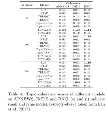
Using the datasets APNEWS, IMDB, and BNC. APNEWS, which is a collection of Associated Press news articles from 2009 to 2016, to do the model evaluation, the paper gets the following result:

• In the evaluation of Language Model:

1. All the topic-enrolled methods outperform the basic-LSTM model, indicating the effectiveness of incorporating global semantic topic information.
2. TCNLM performs the best across all datasets, and the trend keeps improving with the increase of topic numbers.
3. The improved performance of TCNLM over LCLM implies that encoding the document context into meaningful topics provides a better way to improve the language model compared with using the extra context words directly.
4. The margin between LDA+LSTM/Topic-RNN and our TCNLM indicates that our model supplies a more efficient way to utilize the topic information through the joint variational learning framework to implicitly train an ensemble model.

• In the evaluation of Topic Model:

1. TCNLM achieve the best coherence performance over APNEWS and IMDB and are relatively competitive with LDA on BNC.
2. A larger model may result in a slightly worse coherence performance. One possible explanation is that a larger language model may have more impact on the topic model, and the inherited stronger sequential information may be harmful to the coherence measurement.
3. The advantage of TCNLM over Topic-RNN indicates that TCNLM supplies more powerful topic guidance.

Extensions

Another advantage of our TCNLM is its capacity to generate meaningful sentences conditioned on given topics. Significant extensions have proposed, including:

1. Google Mail Smart Compose: Much like autocomplete in the search bar or on your smartphone’s keyboard, the new AI-powered feature promises to not only intelligently work out what you’re currently trying to write but to predict whole emails.
2. Grammarly: Grammarly automatically detects grammar, spelling, punctuation, word choice and style mistakes in your writing.
3. Sentence generator helps people with language barrier express more fluently: Stephen Hawking's main interface to the computer, called ACAT, includes a word prediction algorithm provided by SwiftKey, trained on his books and lectures, so he usually only have to type the first couple of characters before he can select the whole word.