stat946F18/differentiableplasticity: Difference between revisions
(→Model) |
|||
| Line 70: | Line 70: | ||
the full plastic component of the connection. | the full plastic component of the connection. | ||
The network equations are as follows: | The network equations for the output <math display = "inline">x_j(t)</math> of the neuron <math display = "inline">j</math> are as follows: | ||
| Line 83: | Line 83: | ||
</math> | </math> | ||
Here the first equation gives the activation function, where the <math display = "inline">w_{i,j}</math> is a fixed component and the remaining term (<math display = "inline"> \alpha_{i,j} H_{i,j}(t))x_i(t-1) </math>) is a plastic component. The <math display = "inline">\sigma</math> is a nonlinear function. It is always chosen to be tanh in this paper. The <math display = "inline">H_{i,j}</math> in the second equation is updated as a function of ongoing inputs and outputs. | |||
From first equation above, a connection can be fully fixed if <math display = "inline">\alpha = 0 </math> or fully plastic if <math display = "inline">w = 0</math> or have both a fixed and plastic components. | From first equation above, a connection can be fully fixed if <math display = "inline">\alpha = 0 </math> or fully plastic if <math display = "inline">w = 0</math> or have both a fixed and plastic components. | ||
| Line 95: | Line 95: | ||
H_{i,j}(t+1) = H_{i,j}(t) + \eta x_j(t)(x_i(t-1) - x_j(t)H_{i,j}(t)) | H_{i,j}(t+1) = H_{i,j}(t) + \eta x_j(t)(x_i(t-1) - x_j(t)H_{i,j}(t)) | ||
</math> | </math> | ||
= Experiment1 - Binary Pattern Memorization = | = Experiment1 - Binary Pattern Memorization = | ||
Revision as of 22:10, 31 October 2018
Differentiable Plasticity: Summary of the ICML 2018 paper https://arxiv.org/abs/1804.02464
Presented by
1. Ganapathi Subramanian, Sriram [Quest ID: 20676799]
Motivation
1. Neural Networks naturally have a static architecture. Once a Neural Network is trained, the network architecture components (ex. network connections) cannot be changed and effectively learning stops with the training step. If a different task needs to be considered, then the agent must be trained again from scratch.
2. Plasticity is the characteristic of biological systems like humans, which can change network connections over time. This enables lifelong learning in biological systems and thus is capable of adapting to dynamic changes in the environment with great sample efficiency in the data observed. This is called synaptic plasticity which is based on the Hebb's rule (i.e. if a neuron repeatedly takes part in making another neuron fire, the connection between them is strengthened). Neural networks are very far from achieving synaptic plasticity.
3. Differential plasticity is a step in this direction. The plastic connections' behavior is trained using gradient descent so that the previously trained networks can adapt to changing conditions.
Example: Using the current state of the art supervised learning examples, we can train Neural Networks to recognize specific letters that it has seen during training. Using lifelong learning the agent can know about any alphabet, including those that it has never been exposed to during training.
Objectives
The paper has the following objectives:
1. To tackle to problem of meta-learning (learning to learn).
2. To design neural networks with plastic connections with a special emphasis on gradient descent capability for backpropagation training.
3. To use backpropagation to optimize both the base weights and the amount of plasticity in each connection.
4. To demonstrate the performance of such networks on three complex and different domains namely complex pattern memorization, one shot classification and reinforcement learning.
Important Terms
Hebb’s rule: This is a famous rule in neuroscience. It defines the relationship of activities between neurons with their connection. It states that if a neuron repeatedly takes part in making another neuron fire, the connection between them is strengthened. Also summarized as "neurons that fire together, wire together".
Related Work
Previous Approaches to solving this problem are summarized as under:
1. Train standard recurrent neural networks to incorporate past experience in their future responses within each episode. For the learning abilities, the RNN is attached with an external content-addressable memory bank. An attention mechanism within the controller network does the read-write to the memory bank and thus enables fast memorization.

2. Augment each weight with a plastic component that automatically grows and decays as a function of inputs and outputs. All connection have the same non-trainable plasticity and only the corresponding weights are trained. Recent approaches have tried fast-weights which augments recurrent networks with fast-changing Hebbian weights and computes activations at each step. The network has a high bias towards the recently seen patterns.

3. Optimize the learning rule itself instead of the connections. A parametrized learning rule is used where the structure of the network is fixed beforehand.

4. Have all the weight updates to be computed on the fly by the network itself or by a separate network at each time step. Pros are the flexibility and the cons are the large learning burden placed on the network.

5. Perform gradient descent via propagation during the episode. The meta-learning involves training the base network for it to be fine-tuned using additional gradient descent.

6. For classification tasks, a separate embedding is trained to discriminate between different classes. Classification is then a comparison between the embedding of the test and example instances.
The superiority of the trainable synaptic plasticity for the meta-learning approach are as follows:
1. Great potential for flexibility. Example, Memory Networks enforce a specific memory storage model in which memories must be embedded in fixed-size vectors and retrieved through some attention mechanism. In contrast, trainable synaptic plasticity translates into very different forms of memory, the exact implementation of which can be determined by (trainable) network structure.
2. Fixed-weight recurrent networks, meanwhile, require neurons to be used for both storage and computation which increases the computational burdens on neurons. This is avoided in the approach suggested in the paper.
3. Non-trainable plasticity networks can exploit network connectivity for storage of short-term information, but their uniform, non-trainable plasticity imposes a stereotypical behavior on these memories. In the synaptic plasticity, the amount and rate of plasticity are actively molded by the mechanism itself. Also, it allows for more sustained memory.
Model
The formulation proposed in the paper is in such a way that the plastic and non-plastic components for each connection are kept separate, while multiple Hebbian rules can be easily defined.
Model Components:
1. A connection between any two neurons [math]\displaystyle{ i }[/math] and [math]\displaystyle{ j }[/math] has both a fixed component and a plastic component.
2. The fixed part is just a traditional connection weight [math]\displaystyle{ w_{i,j} }[/math] . The plastic part is stored in a Hebbian trace [math]\displaystyle{ H_{i,j} }[/math], which varies during a lifetime according to ongoing inputs and outputs.
3. The relative importance of plastic and fixed components in the connection is structurally determined by the plasticity coefficient [math]\displaystyle{ \alpha_{i,j} }[/math], which multiplies the Hebbian trace to form the full plastic component of the connection.
The network equations for the output [math]\displaystyle{ x_j(t) }[/math] of the neuron [math]\displaystyle{ j }[/math] are as follows:
[math]\displaystyle{
x_j(t) = \sigma{\displaystyle \sum_{i \in \text{inputs}}[(w_{i,j}x_i(t-1) + \alpha_{i,j} H_{i,j}(t))x_i(t-1)] }
}[/math]
[math]\displaystyle{ H_{i,j}(t+1) = \eta x_i(t-1) x_j(t) + (1 - \eta) H_{i,j}(t) }[/math]
Here the first equation gives the activation function, where the [math]\displaystyle{ w_{i,j} }[/math] is a fixed component and the remaining term ([math]\displaystyle{ \alpha_{i,j} H_{i,j}(t))x_i(t-1) }[/math]) is a plastic component. The [math]\displaystyle{ \sigma }[/math] is a nonlinear function. It is always chosen to be tanh in this paper. The [math]\displaystyle{ H_{i,j} }[/math] in the second equation is updated as a function of ongoing inputs and outputs.
From first equation above, a connection can be fully fixed if [math]\displaystyle{ \alpha = 0 }[/math] or fully plastic if [math]\displaystyle{ w = 0 }[/math] or have both a fixed and plastic components.
The terms [math]\displaystyle{ w_{i,j} }[/math] and [math]\displaystyle{ \alpha_{i,j} }[/math] are the structural parameters trained by gradient descent. The [math]\displaystyle{ \eta }[/math] which denotes the learning rate is also an optimized parameter of the network. After this training, the agent can learn automatically from ongoing experience. In equation 2 above, the [math]\displaystyle{ \eta }[/math] could make the Hebbian traces to decay to 0 in the absence of input. So another form of the equation is as follows:
[math]\displaystyle{
H_{i,j}(t+1) = H_{i,j}(t) + \eta x_j(t)(x_i(t-1) - x_j(t)H_{i,j}(t))
}[/math]
Experiment1 - Binary Pattern Memorization
This test involves quickly memorizing sets of arbitrary high-dimensional patterns and reconstructing the same while being exposed to partial, degraded versions of them. This is a very simple test as it is already known that hand designed recurrent networks with a Hebbian plastic connection can already solve it for binary patterns.
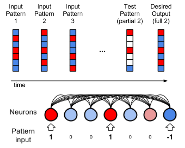
Steps in the experiment:
1) The network is a set of five binary patterns in succession as shown in the figure 1. Each of these patterns has 1000 elements each of which has one of the binary value (1 or -1). Here 1 corresponds to dark red and -1 corresponds to dark blue.
2) The few shot learning paradigm is followed, where each pattern is shown for 10-time steps, with 3-time steps of zero input between the presentations and the whole sequence of patterns is presented 3 times in random order.
3) One of the presented patterns is chosen in random order and degraded by setting half of its bits to 0.
4) This degraded pattern is then fed to the network. The network has to reproduce the correct full pattern in its output using its memory that it developed during training.
The architecture of the network is described as follows:
1) It is a fully connected RNN with one neuron per pattern element, plus one fixed-output neuron. There are a total of 1001 neurons.
2) Value of each neuron is clamped to the value of the corresponding element in the pattern if the value is not 0. If the value is 0, the corresponding neurons do not receive pattern input and must use what it gets from lateral connections and reconstruct the correct, expected output values.
3) Outputs are read from the activation of the neurons.
4) The performance evaluation is done by computing the loss between the final network output and the correct expected pattern.
5) The gradient of the error over the [math]\displaystyle{ w_{i,j} }[/math] and the [math]\displaystyle{ \alpha_{i,j} }[/math] coefficients is computed by backpropagation and optimized through Adam solver with learning rate 0.001.
6) The simple decaying Hebbian formula in Equation 2 is used to update the Hebbian traces. Each network has 2 trainable parameters [math]\displaystyle{ w }[/math] and [math]\displaystyle{ \alpha }[/math] for each connection, thus there are a total 1001 [math]\displaystyle{ \times }[/math] 1001 [math]\displaystyle{ \times }[/math] 2 = 2004002 trainable parameters.
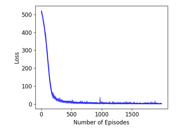
The results are shown in the figure 2 where 10 runs are considered. The error becomes quite low after about 200 episodes of training.
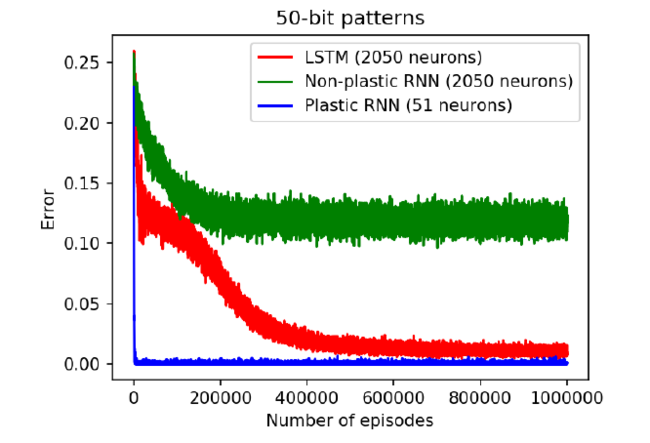
Comparison with Non-Plastic Networks:
1) Nonplastic networks can solve this task but require additional neurons to solve this task in principle. In practice, the authors say that the task is not solved using Non-plastic RNN or LSTM.
2) The figure 3 shows the results using non-plastic networks. The best results required the addition of 2000 extra neurons.
3) For non-plastic RNN, the error flattens around 0.13 which is quite high. Using LSTMs, the task can be solved albeit imperfectly and also the error rate reduces drastically t0 around 0.001.
4) The plastic network solves the task very quickly with the mean error going below 0.01 within 2000 episodes which are mentioned to be 250 times faster than the LSTM.
Experiment2 - Memorizing network images
This task is an image reconstruction task that where a network is trained on a set of natural images which it looks to memorize. The natural images with graded pixel values contain more information per element as compared to the last experiment. So this experiment is inherently more complex than the previous ones. Then one image is chosen at random and half the image is displayed to the agent. The task is to complete the image. The paper shows that this method effectively solves this task which other state-of-the-art network architectures fail to solve.
The experiment is as follows:
1) Images are from the CIFAR-10 database where there are a total of 60000 images each of size 32 [math]\displaystyle{ \times }[/math] 32.
2) The architecture has 1025 neurons in total with a total of 2 [math]\displaystyle{ \times }[/math] 1025 [math]\displaystyle{ \times }[/math] 1025 = 2101250 parameters.
3) Each episode has 3 pictures, shown 3 times for 20-time steps each time, with 3-time steps of zero input between the presentations.
4) The images are degraded by zeroing out one full contiguous half of the image to prevent a trivial solution of simply reconstructing the missing pixel as the average of its neighbors.
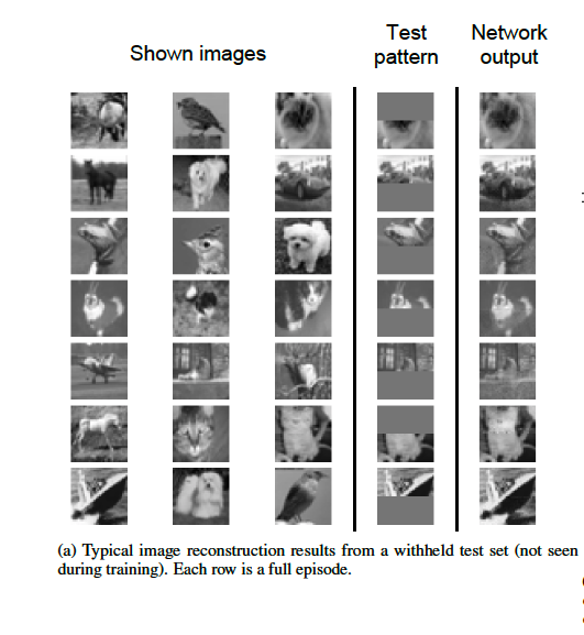
The results are shown in figure 4. The final output of the network is shown in the last column which is the reconstructed image. The results show that the model has learned to perform this task.
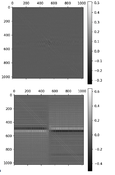
The final weight matrix and plasticity coefficients matrix are shown in the figure 5. The plasticity matrix shows a structure related to the high correlation of neighboring pixels and half-field zeroing in test images.
The full plastic network is compared against a similar architecture with shared plasticity coefficients, where all connections share the same [math]\displaystyle{ \alpha }[/math] value. So, the single parameter is shared across all connections is trained.
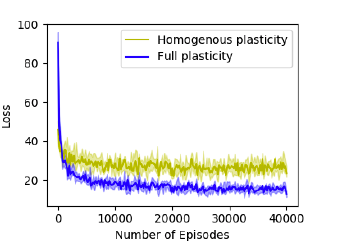
The figure 6 shows the result of comparison where the independent plasticity coefficient for each connection has better performances. Thus the structure observed in the weight matrices of the results is actually useful.
Experiment 3 - Omniglot task
This task involves handwritten symbol recognition. It is a standard task for one-shot and few-shot learning.
Experimental Setup:
1) The Omniglot data set is a collection of handwritten characters from various writing systems, including 20 instances each of 1,623 different handwritten characters, written by different subjects.
2) In each episode, N character classes are randomly selected and K instances from each class are sampled.
3) These instances, together with the class label (from 1 to N), are shown to the model.
4) Then, a new, unlabelled instance is sampled from one of the N classes and shown to the model.
5) Model performance is defined as the model’s accuracy in classifying this unlabelled example.
Architecture:
1) Model architecture has 4 convolutional layers with 3 [math]\displaystyle{ \times }[/math] 3 receptive fields and 64 channels.
2) All convolutions have a stride of 2 to reduce the dimensionality between layers.
3) The output is a single vector of 64 features, which feeds into an N-way softmax.
4) The label of the current character is also concurrently fed as a one-hot encoding to this softmax layer, to serve as a guide for the correct output when a label is present.
Plasticity in the architecture:
1) Plasticity is applied to the weights from the final layer to the softmax layer, leaving the rest of the convolutional embedding non- plastic.
2) The expectation is that the convolutional architecture will learn an adequate discriminant between arbitrary handwritten characters and the plastic weights learns to memorize associations between observed patterns and outputs.
Data Preparation:
1) The dataset is augmented with rotations by multiples of [math]\displaystyle{ 90 }[/math] degrees.
2) It is divided into 1,523 classes for training and 100 classes (together with their augmentations) for testing.
3) The networks are trained with an Adam optimizer with a learning rate 3 [math]\displaystyle{ \times 10^{-5} }[/math], multiplied by 2/3 every 1M episodes over 5,000,000 episodes.
4) To evaluate final model performance, 10 models are trained with different random seeds and each of those is tested on 100 episodes using previously unseen test classes.
Results:
1) The overall accuracy (i.e. the proportion of episodes with correct classification, aggregated over all test episodes of all runs) is 98.3%, with a 95% confidence interval of 0.80%.
2) The median accuracy across the 10 runs was 98.5%, indicating consistency in learning.
| Memory Networks | Matching Networks | ProtoNets | Memory Module | MAML | SNAIL | DP(This paper) |
|---|---|---|---|---|---|---|
| 82.8% | 98.1% | 97.4% | 98.4% | 98.7% [math]\displaystyle{ \pm }[/math] 0.4 | 99.07% [math]\displaystyle{ \pm }[/math] 0.16 | 98.03% [math]\displaystyle{ \pm }[/math] 0.80 |
3) The above table shows the comparative performance across other non-plastic approaches. The results of the plastic approach are largely similar to those reported for the computationally intensive MAML method and the classification-specialized Matching Networks method.
4) The performances are slightly below those reported for the SNAIL method, which trains a whole additional temporal-convolution network on top of the convolutional architecture thus having many more parameters.
5) The conclusion is that a few plastic connections to the output of the network allow for competitive one-shot learning over arbitrary man-made visual symbols.
This is a maze exploration task where the goal is to teach an agent to reach a goal. The plastic networks are shown to outperform non-plastic ones.
Experimental setup:
1) The maze is composed of 9 [math]\displaystyle{ \times }[/math] 9 squares, surrounded by walls, in which every other square (in either direction) is occupied by a wall.
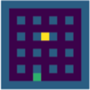
2) The maze contains 16 wall square arranged in a regular grid as shown in the figure 7.
3) At each episode, one non-wall square is randomly chosen as the reward location. When the agent hits this location, it receives a large reward (10.0) and is immediately transported to a random location in the maze Also a small negative reward of -0.1 is provided every time the agent tries to walk into a wall).
4) Each episode lasts 250-time steps, during which the agent must accumulate as much reward as possible. The reward location is fixed within an episode and randomized across episodes.
5) The reward is invisible to the agent, and thus the agent only knows it has hit the reward location by the activation of the reward input at the next step.
6) Inputs to the agent consist of a binary vector describing the 3 [math]\displaystyle{ \times }[/math] 3 neighborhood centered on the agent (each element being set to 1 or 0 if the corresponding square is or is not a wall), together with the reward at the previous time step.
7) A2C algorithm is used to meta train the network.
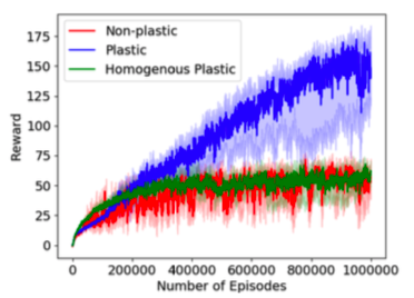
8) The experiments are run under three conditions: full differentiable plasticity, no plasticity at all, and homogeneous plasticity in which all connections share the same (learnable) [math]\displaystyle{ \alpha }[/math] parameter.
9) For each condition, 15 runs with different random seeds are performed.
Architecture:
1) It is a simple recurrent network with 200 neurons, with a softmax layer on top of it to select between the 4 possible actions (up, right, left or down).
Results:
1) The results are shown in the figure 8. The plastic network shows considerably better performance as compared to the other networks.
2) The non-plastic and homogeneous networks get stuck on a suboptimal policy.
3) Thus, the conclusion is that, in this domain, individually sculpting the plasticity of each connection is crucial in reaping the benefits of plasticity for this task.
Conclusions
The important contributions from this paper are as follows:
1) The results show that simple plastic models support efficient meta-learning.
2) Gradient descent itself is shown to be capable of optimizing the plasticity of a meta-learning system.
3) The meta-learning is shown to vastly outperform alternative options in the experiments considered.
4) The method achieved state of the art results on a hard Omniglot test set.
Open Source Code
Code for this paper can be found at: https://github.com/uber-common/differentiable-plasticity
Critiques
The paper addresses an important problem of learning to learn ("meta-learning") and provides a novel framework based on gradient descent to achieve this objective. This paper provides a large scope for future work as many widely used architectures like LSTMs could be tried along with a plastic component. It is also easy to see that the application of such approaches in deep reinforcement learning are also plentiful and there is a good possibility of beating the current baselines in many popular test beds like Atari games using plastic networks. This paper opens up possibilities for a whole class of meta-learning algorithms.
With regards to the drawbacks of the paper, the paper does not mention how plastic networks will behave if the test sets are completely different from the training dataset. Will the performance be the same as non-plastic networks? It is not very clear if this method will be scalable as there are a large number of parameters to be determined even with the simplest of problems. Also, each experimental domain considered in this paper needed significantly different network architectures (for example in the Omniglot domain plasticity was applied only for the final layers). The paper does not mention any reasons for the specific decisions and if such differences will hold good for other similar problems as well. There has been work in transfer learning applied to both supervised learning and reinforcement learning problems. The authors should have ideally compared plastic networks to performances of some algorithms there as these methods transfer existing knowledge to other related problems and also prevent the need to start training from scratch much similar to the methods adopted in this paper.