Wavelet Pooling CNN: Difference between revisions
(fixed backpropogation description) |
|||
| Line 9: | Line 9: | ||
[[File:WT_Fig1.PNG|650px|center|]] | [[File:WT_Fig1.PNG|650px|center|]] | ||
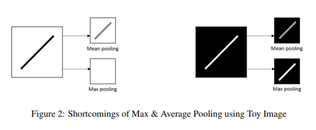
The paper mentions that these pooling methods, although simple and effective, have shortcomings. Max pooling can omit details from an image if the important features have less intensity than the insignificant ones, and also commonly overfits. On the other hand, average pooling can dilute important features if the data is averaged with values of significantly lower intensities. Figure 2 displays an image of this. | The paper mentions that these pooling methods, although simple and effective, have shortcomings. Max pooling can omit details from an image if the important features have less intensity than the insignificant ones (unless the neural network has learnt to inverse the intensity level), and also commonly overfits. On the other hand, average pooling can dilute important features if the data is averaged with values of significantly lower intensities. Figure 2 displays an image of this. | ||
[[File:WT_Fig2.PNG|650px|center|]] | [[File:WT_Fig2.PNG|650px|center|]] | ||
Revision as of 18:07, 18 April 2018
Introduction
Convolutional neural networks (CNN) have been proven to be powerful in image classification. Over the past few years, researchers have put efforts in improving fundamental components of CNNs such as the pooling operation. Various pooling methods exist; deterministic methods include max pooling and average pooling and probabilistic methods include mixed pooling and stochastic pooling. All these methods employ a neighborhood approach to the sub-sampling which, albeit fast and simple, can produce artifacts such as blurring, aliasing, and edge halos (Parker et al., 1983).
This paper introduces a novel pooling method based on the discrete wavelet transform. Specifically, it uses a second-level wavelet decomposition for the sub-sampling. This method, instead of nearest neighbor interpolation uses a sub-band method that the authors' claim produces fewer artifacts and represents the underlying features more accurately. Therefore, if pooling is viewed as a lossy process, the reason for employing a wavelet approach is to try to minimize this loss.
Pooling Background
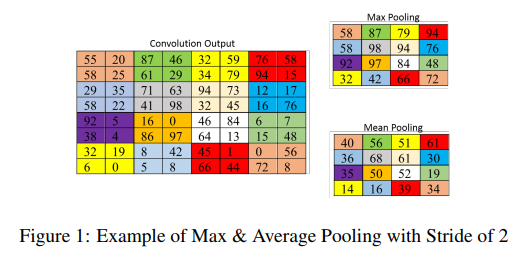
Pooling essentially means sub-sampling. After the pooling layer, the spatial dimensions of the data is reduced to some degree, with the goal being to compress the data rather than discard some of it. Typical approaches to pooling reduce the dimensionality by using some method to combine a region of values into one value. Max pooling and Mean/Average pooling are the 2 most commonly used pooling methods. For max pooling, this can be represented by the equation [math]\displaystyle{ a_{kij} = max_{(p,q) \epsilon R_{ij}} (a_{kpq}) }[/math] where [math]\displaystyle{ a_{kij} }[/math] is the output activation of the [math]\displaystyle{ k^th }[/math] feature map at [math]\displaystyle{ (i,j) }[/math], [math]\displaystyle{ a_{kpq} }[/math] is input activation at [math]\displaystyle{ (p,q) }[/math] within [math]\displaystyle{ R_{ij} }[/math], and [math]\displaystyle{ |R_{ij}| }[/math] is the size of the pooling region. Mean pooling can be represented by the equation [math]\displaystyle{ a_{kij} = \frac{1}{|R_{ij}|} \sum_{(p,q) \epsilon R_{ij}} (a_{kpq}) }[/math] with everything defined as before. Figure 1 provides a numerical example that can be followed.
The paper mentions that these pooling methods, although simple and effective, have shortcomings. Max pooling can omit details from an image if the important features have less intensity than the insignificant ones (unless the neural network has learnt to inverse the intensity level), and also commonly overfits. On the other hand, average pooling can dilute important features if the data is averaged with values of significantly lower intensities. Figure 2 displays an image of this.
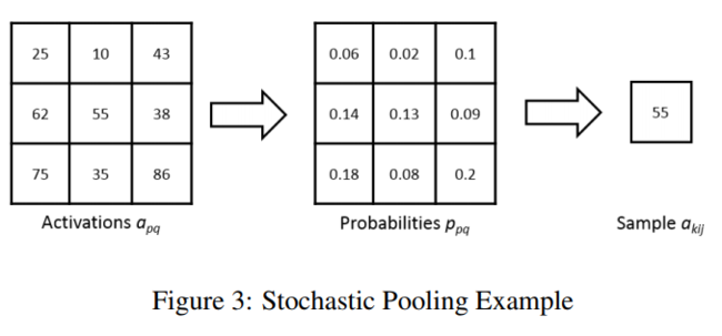
To account for the above-mentioned issues, probabilistic pooling methods were introduced, namely mixed pooling and; stochastic pooling. Mixed pooling is a simple method which just combines the max and the average pooling by randomly selecting one method over the other during training. Mixed pooling can be applied for all features, mixed between features, or mixed between regions for different features. Stochastic pooling on the other hand randomly samples within a receptive field with the activation values as the probabilities. These are calculated by taking each activation value and dividing it by the sum of all activation values in the grid so that the probabilities sum to 1.
Figure 3 shows an example of how stochastic pooling works. On the left is a 3x3 grid filled with activations. The middle grid is the corresponding probability for each activation. The activation in the middle was randomly selected (it had a 13% chance of getting selected). Because the stochastic pooling is based on the probability of the pixels, it is able to avoid the shortcomings of max and mean pooling mentioned above.
Wavelet Background
Data or signals tend to be composed of slowly changing trends (low frequency) as well as fast-changing transients (high frequency). Similarly, images have smooth regions of intensity which are perturbed by edges or abrupt changes. We know that these abrupt changes can represent features that are of great importance to us when we perform deep learning. Wavelets are a class of functions that are well localized in time and frequency. The wavelet transform is often compared with the Fourier transform, in which signals are represented as a sum of sinusoids. In fact, the Fourier transform can be viewed as a special case of the continuous wavelet transform with the choice of the mother wavelet [math]\displaystyle{ \psi(t)=e^{-2 \pi it} }[/math]. The main difference in general is that wavelets are localized in both time and frequency whereas the standard Fourier transform is only localized in frequency. The ability of wavelets to be localized in time and space is what makes it suitable for detecting the abrupt changes in an image well.
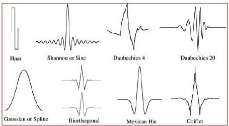
Essentially, a wavelet is a fast decaying oscillating signal with zero mean that only exists for a fixed duration and can be scaled and shifted in time. There are some well-defined types of wavelets as shown in Figure 3. The key characteristic of wavelets for us is that they have a band-pass characteristic, and the band can be adjusted based on the scaling and shifting.
The paper uses discrete wavelet transform and more specifically a faster variation called Fast Wavelet Transform (FWT) using the Haar wavelet. There also exists a continuous wavelet transform. The main difference in these is how the scale and shift parameters are selected.
Discrete Wavelet Transform General
The discrete wavelet transforms for images is essentially applying a low pass and high pass filter to your image where the transfer functions of the filters are related and defined by the type of wavelet used (Haar in this paper). This is shown in the figures below, which also show the recursive nature of the transform. For an image, the per-row transform is taken first. This results in a new image where the first half is a low-frequency sub-band and the second half is the high-frequency sub-band. Then this new image is transformed again per column, resulting in four sub-bands. Generally, the low-frequency content approximates the image and the high-frequency content represents abrupt changes. Therefore, one can simply take the LL band and perform the transformation again to sub-sample even more.

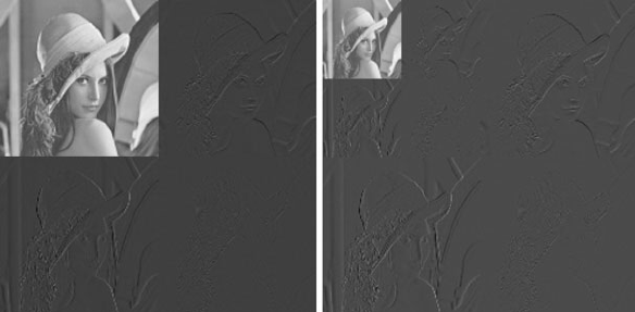
In left half of the above image we see a grid containing four different transformations of the same initial image. Each transform has been done by applying a row wise convolution with a wavelet of either high or low frequency, then a column wise convolution with another wavelet of either high or low frequency. The four choices of frequency (LL, LH, HL, HH) result in four different images. The top left image is the result of applying a low frequency wavelet convolution to the original image both row wise and column wise. The bottom left image is the result of first applying a high frequency wavelet convolution row wise and then applying a low frequency wavelet convolution column wise. Since the LL (top right) transformation preserves the original image best, it is then used in this process again to generate the grid of smaller images that can be seen in the top center-right of the above image. The images in this smaller grid are called second order coefficients.
DWT example using Haar Wavelet
Suppose we have an image represented by the following pixels:
\begin{align} \begin{bmatrix} 100 & 50 & 60 & 150 \\ 20 & 60 & 40 & 30 \\ 50 & 90 & 70 & 82 \\ 74 & 66 & 90 & 58 \\ \end{bmatrix} \end{align}
For each level of the DWT using the Haar wavelet, we will perform the transform on the rows first and then the columns. For the row pass, we transform each row as follows:
- For each row i = [math]\displaystyle{ [i_{1}, i_{2}, i_{3}, i_{4}] }[/math] of the input image, transform the row to [math]\displaystyle{ i_{t} }[/math] via
\begin{align} i_{t} = [(i_{1} + i_{2}) / 2, (i_{3} + i_{4}) / 2, (i_{1}, - i_{2}) / 2, (i_{3} - i_{4}) / 2] \end{align}
After the row transforms, the images looks as follows: \begin{align} \begin{bmatrix} 75 & 105 & 25 & -45 \\ 40 & 35 & -20 & 5 \\ 70 & 76 & -20 & -6 \\ 70 & 74 & 4 & 16 \\ \end{bmatrix} \end{align}
Now we apply the same method to the columns in the exact same way.
Proposed Method
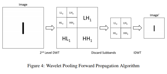
The proposed method uses subbands from the second level FWT and discards the first level subbands. The authors postulate that this method is more 'organic' in capturing the data compression and will create less artifacts that may affect the image classification.
Forward Propagation
FWT can be expressed by [math]\displaystyle{ W_\varphi[j + 1, k] = h_\varphi[-n]*W_\varphi[j,n]|_{n = 2k, k \lt = 0} }[/math] and [math]\displaystyle{ W_\psi[j + 1, k] = h_\psi[-n]*W_\psi[j,n]|_{n = 2k, k \lt = 0} }[/math] where [math]\displaystyle{ \varphi }[/math] is the approximation function, [math]\displaystyle{ \psi }[/math] is the detail function, [math]\displaystyle{ W_\varphi }[/math], [math]\displaystyle{ W_\psi }[/math], are approximation and detail coefficients, [math]\displaystyle{ h_\varphi[-n] }[/math] and [math]\displaystyle{ h_\psi[-n] }[/math] are time reversed scaling and wavelet vectors, [math]\displaystyle{ (n) }[/math] represents the sample in the vector, and [math]\displaystyle{ j }[/math] denotes the resolution level. To apply to images, FWT is first applied on the rows and then the columns. If a low (L) and high(H) sub-band is extracted from the rows and similarly for the columns than at each level there is 4 sub-bands (LH, HL, HH, and LL) where LL will further be decomposed into the level 2 decomposition.
Using the level 2 decomposition sub-bands, the Inverse Fast Wavelet Transform (IFWT) is used to obtain the resulting sub-sampled image, which is sub-sampled by a factor of two. The Equation for IFWT is [math]\displaystyle{ W_\varphi[j, k] = h_\varphi[-n]*W_\varphi[j + 1,n] + h_\psi[-n]*W_\psi[j + 1,n]|_{n = \frac{k}{2}, k \lt = 0} }[/math] where the parameters are the same as previously explained. Figure 4 displays the algorithm for the forward propagation.
Back Propagation
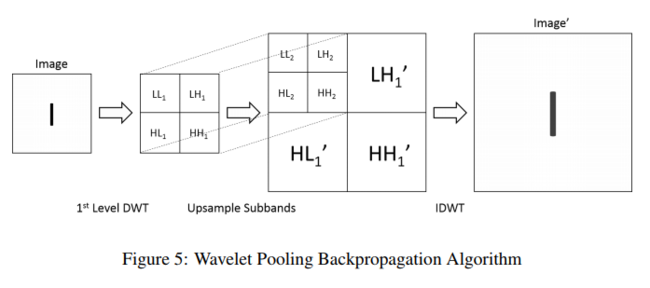
This is simply the reverse of the forward propagation. The image feature first has to be converted into the sub-bands using the 1st order wavelet decomposition. The sub-bands are upsampled by a factor of 2 and then backpropagated through the IDWT to achieve the final image. Figure 5 displays the algorithm.
Results
The authors tested on MNIST, CIFAR-10, SHVN, and KDEF and the paper provides comprehensive results for each. Stochastic gradient descent was used and the Haar wavelet is used due to its even, square subbands. The network for all datasets except MNIST is loosely based on (Zeiler & Fergus, 2013). The authors keep the network consistent but change the pooling method for each dataset. They also experiment with dropout and Batch Normalization to examine the effects of regularization on their method. All pooling methods compared use a 2x2 window, and a consistent pooling method was used for all pooling layers of a network. The overall results teach us that the pooling method should be chosen specifically for the type of data we have. In some cases, wavelet pooling may perform the best, and in other cases, other methods may perform better, if the data is more suited for those types of pooling.
MNIST
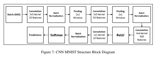
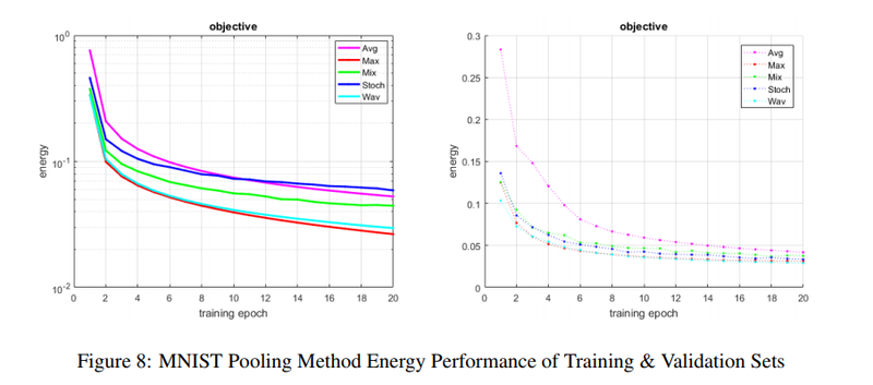
Figure 7 shows the network how's architecture was based on an example of MNIST structure from MatConvNet, with batch normalization. Table 1 shows the algorithms accuracy. It can be seen that wavelet pooling achieves the best accuracy from all pooling methods compared. Figure 8 shows the energy of each method per epoch. As can be noted by Figure 8 average and wavelet pooling show a smoother descent in learning and error reduction.

CIFAR-10
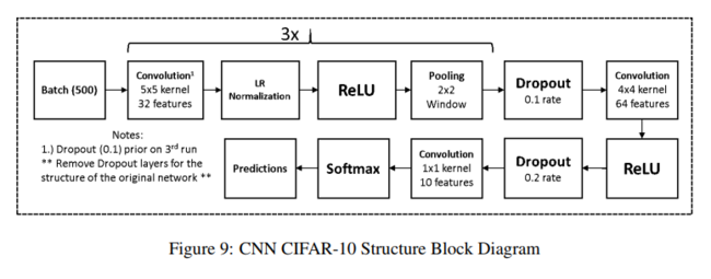
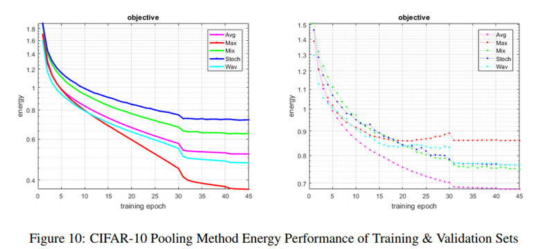
In order to investigate the performance of different pooling methods, two types of networks are trained based on CIFAR-10. The first one is the regular CNN and the second one is the network with dropout and batch normalization. Figure 9 shows the network and Tables 2 and 3 shows the accuracy without and with dropout. Average pooling achieves the best accuracy but wavelet pooling is still competitive, while max pooling overfitted on the validation data fairly quickly as shown by the right energy curve in Figure 10 (although the accuracy performance is not significantly worse when dropout and batch normalization are applied).


SHVN
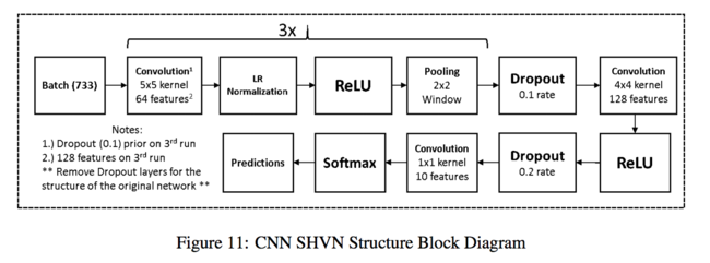
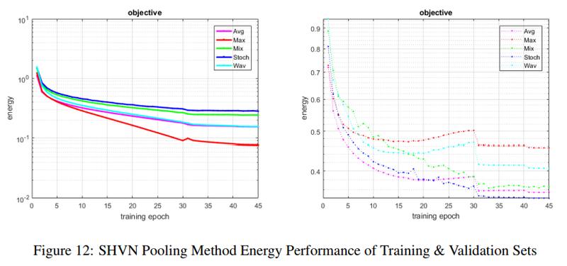
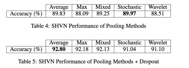
Figure 11 shows the network and Tables 4 and 5 shows the accuracy without and with dropout. The proposed method does not perform well in this experiment.
KDEF
The authors experimented with pooling methods + dropout on the KDEF dataset (which consists of 4,900 images of 35 people portraying varying emotions through facial expressions under different poses, 3,900 of which were randomly assigned to be used for training). The data was treated for errors (e.g. corrupt images) and resized to 128x128 for memory and time constraints.
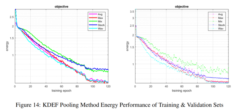
Figure 13 below shows the network structure. Figure 14 shows the energy curve of the competing models on training and validation sets as the number of epochs increases, and Table 6 shows the accuracy performance. Average pooling demonstrated the highest accuracy, with wavelet pooling coming in second and max-pooling a close third. However, stochastic and wavelet pooling exhibited more stable learning progression compared to the other methods, and max-pooling eventually overfitted.


Computational Complexity
The authors explain that their paper is a proof of concept and is not meant to implement wavelet pooling in the most efficient way. The table below displays a comparison of the number of mathematical operations for each method according to the dataset. It can be seen that wavelet pooling is significantly worse. The authors explain that through good implementation and coding practices, the method can prove to be viable.

Criticism
Positive
- Wavelet Pooling achieves competitive performance with standard go-to pooling methods
- Leads to a comparison of discrete transformation techniques for pooling (DCT, DFT)
Negative
- Only 2x2 pooling window used for comparison
- Highly computationally extensive
- Not as simple as other pooling methods
- Only one wavelet used (HAAR wavelet)
References
- Travis Williams and Robert Li. Wavelet Pooling for Convolutional Neural Networks. ICLR 2018.
- J. Anthony Parker, Robert V. Kenyon, and Donald E. Troxel. Comparison of interpolating methods for image resampling. IEEE Transactions on Medical Imaging, 2(1):31–39, 1983.
- Matthew Zeiler and Robert Fergus. Stochastic pooling for regularization of deep convolutional neural networks. In Proceedings of the International Conference on Learning Representation (ICLR), 2013.