MarrNet: 3D Shape Reconstruction via 2.5D Sketches

Introduction

Humans are able to quickly recognize 3D shapes from images, even in spite of drastic differences in object texture, material, lighting, and background.

Objects in real images. The appearance of the same shaped object varies based on colour, texture, lighting, background, etc. However, the 2.5D sketches (e.g. depth or normal maps) of the object remain constant, and can be seen as an abstraction of the object which is used to reconstruct the 3D shape.

In this work, the authors propose a novel end-to-end trainable model that sequentially estimates 2.5D sketches and 3D object shape from images and also enforce the re projection consistency between the 3D shape and the estimated sketch. The two step approach makes the network more robust to differences in object texture, material, lighting and background. Based on the idea from [Marr, 1982] that human 3D perception relies on recovering 2.5D sketches, which include depth maps (contains information related to the distance of surfaces from a viewpoint) and surface normal maps (technique for adding the illusion of depth details to surfaces using an image's RGB information), the authors design an end-to-end trainable pipeline which they call MarrNet. MarrNet first estimates depth, normal maps, and silhouette, followed by a 3D shape. MarrNet uses an encoder-decoder structure for the sub-components of the framework.

The authors claim several unique advantages to their method. Single image 3D reconstruction is a highly under-constrained problem, requiring strong prior knowledge of object shapes. As well, accurate 3D object annotations using real images are not common, and many previous approaches rely on purely synthetic data. However, most of these methods suffer from domain adaptation due to imperfect rendering.

Using 2.5D sketches can alleviate the challenges of domain transfer. It is straightforward to generate perfect object surface normals and depths using a graphics engine. Since 2.5D sketches contain only depth, surface normal, and silhouette information, the second step of recovering 3D shape can be trained purely from synthetic data. As well, the introduction of differentiable constraints between 2.5D sketches and 3D shape makes it possible to fine-tune the system, even without any annotations.

The framework is evaluated on both synthetic objects from ShapeNet, and real images from PASCAL 3D+, showing good qualitative and quantitative performance in 3D shape reconstruction.

Related Work

2.5D Sketch Recovery

Researchers have explored recovering 2.5D information from shading, texture, and colour images in the past. More recently, the development of depth sensors has led to the creation of large RGB-D datasets, and papers on estimating depth, surface normals, and other intrinsic images using deep networks. While this method employs 2.5D estimation, the final output is a full 3D shape of an object.

Results from the paper: Learning Non-Lambertian Object Intrinsics across ShapeNet Categories. The results show that neural networks can be trained to recover 2.5D information from an image. The top row predicts the albedo and the bottom row predicts the shading. It can be observed that the results are still blurry and the fine details are not fully recovered.

Single Image 3D Reconstruction

The development of large-scale shape repositories like ShapeNet has allowed for the development of models encoding shape priors for single image 3D reconstruction. These methods normally regress voxelized 3D shapes, relying on synthetic data or 2D masks for training. A voxel is an abbreviation for volume element, the three-dimensional version of a pixel. The formulation in the paper tackles domain adaptation better, since the network can be fine-tuned on images without any annotations.

2D-3D Consistency

Intuitively, the 3D shape can be constrained to be consistent with 2D observations. This idea has been explored for decades, with the use of depth and silhouettes, as well as some papers enforcing differentiable 2D-3D constraints for joint training of deep networks. In this work, this idea is exploited to develop differentiable constraints for consistency between the 2.5D sketches and 3D shape.

Approach

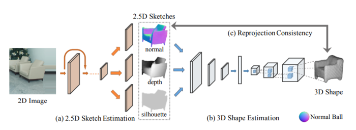
The 3D structure is recovered from a single RGB view using three steps, shown in the figure below. The first step estimates 2.5D sketches, including depth, surface normal, and silhouette of the object. The second step estimates a 3D voxel representation of the object. The third step uses a reprojection consistency function to enforce the 2.5D sketch and 3D structure alignment.

MarrNet architecture. 2.5D sketches of normals, depths, and silhouette are first estimated. The sketches are then used to estimate the 3D shape. Finally, re-projection consistency is used to ensure consistency between the sketch and 3D output.

2.5D Sketch Estimation

The first step takes a 2D RGB image and predicts the 2.5 sketch with surface normal, depth, and silhouette of the object. The goal is to estimate intrinsic object properties from the image, while discarding non-essential information such as texture and lighting. An encoder-decoder architecture is used. The encoder is a A ResNet-18 network, which takes a 256 x 256 RGB image and produces 512 feature maps of size 8 x 8. The decoder is four sets of 5 x 5 convolutional and ReLU layers, followed by four sets of 1 x 1 convolutional and ReLU layers. The output is 256 x 256 resolution depth, surface normal, and silhouette images.

3D Shape Estimation

The second step estimates a voxelized 3D shape using the 2.5D sketches from the first step. The focus here is for the network to learn the shape prior that can explain the input well, and can be trained on synthetic data without suffering from the domain adaptation problem since it only takes in surface normal and depth images as input. The network architecture is inspired by the TL network, and 3D-VAE-GAN, with an encoder-decoder structure. The normal and depth image, masked by the estimated silhouette, are passed into 5 sets of convolutional, ReLU, and pooling layers, followed by two fully connected layers, with a final output width of 200. The 200-dimensional vector is passed into a decoder of 5 convolutional and ReLU layers, outputting a 128 x 128 x 128 voxelized estimate of the input.

Re-projection Consistency

The third step consists of a depth re-projection loss and surface normal re-projection loss. Here, [math]\displaystyle{ v_{x, y, z} }[/math] represents the value at position [math]\displaystyle{ (x, y, z) }[/math] in a 3D voxel grid, with [math]\displaystyle{ v_{x, y, z} \in [0, 1] ∀ x, y, z }[/math]. [math]\displaystyle{ d_{x, y} }[/math] denotes the estimated depth at position [math]\displaystyle{ (x, y) }[/math], [math]\displaystyle{ n_{x, y} = (n_a, n_b, n_c) }[/math] denotes the estimated surface normal. Orthographic projection is used.

Reprojection consistency for voxels. Left and middle: criteria for depth and silhouettes. Right: criterion for surface normals

Depths

The voxel with depth [math]\displaystyle{ v_{x, y}, d_{x, y} }[/math] should be 1, while all voxels in front of it should be 0. This ensures the estimated 3D shape matches the estimated depth values. The projected depth loss and its gradient are defined as follows:

[math]\displaystyle{ L_{depth}(x, y, z)= \left\{ \begin{array}{ll} v^2_{x, y, z}, & z \lt d_{x, y} \\ (1 - v_{x, y, z})^2, & z = d_{x, y} \\ 0, & z \gt d_{x, y} \\ \end{array} \right. }[/math]

[math]\displaystyle{ \frac{∂L_{depth}(x, y, z)}{∂v_{x, y, z}} = \left\{ \begin{array}{ll} 2v{x, y, z}, & z \lt d_{x, y} \\ 2(v_{x, y, z} - 1), & z = d_{x, y} \\ 0, & z \gt d_{x, y} \\ \end{array} \right. }[/math]

When [math]\displaystyle{ d_{x, y} = \infty }[/math], all voxels in front of it should be 0.

Surface Normals

Since vectors [math]\displaystyle{ n_{x} = (0, −n_{c}, n_{b}) }[/math] and [math]\displaystyle{ n_{y} = (−n_{c}, 0, n_{a}) }[/math] are orthogonal to the normal vector [math]\displaystyle{ n_{x, y} = (n_{a}, n_{b}, n_{c}) }[/math], they can be normalized to obtain [math]\displaystyle{ n’_{x} = (0, −1, n_{b}/n_{c}) }[/math] and [math]\displaystyle{ n’_{y} = (−1, 0, n_{a}/n_{c}) }[/math] on the estimated surface plane at [math]\displaystyle{ (x, y, z) }[/math]. The projected surface normal tried to guarantee voxels at [math]\displaystyle{ (x, y, z) ± n’_{x} }[/math] and [math]\displaystyle{ (x, y, z) ± n’_{y} }[/math] should be 1 to match the estimated normal. The constraints are only applied when the target voxels are inside the estimated silhouette.

The projected surface normal loss is defined as follows, with [math]\displaystyle{ z = d_{x, y} }[/math]:

[math]\displaystyle{ L_{normal}(x, y, z) = (1 - v_{x, y-1, z+\frac{n_b}{n_c}})^2 + (1 - v_{x, y+1, z-\frac{n_b}{n_c}})^2 + (1 - v_{x-1, y, z+\frac{n_a}{n_c}})^2 + (1 - v_{x+1, y, z-\frac{n_a}{n_c}})^2 }[/math]

Gradients along x are:

[math]\displaystyle{ \frac{dL_{normal}(x, y, z)}{dv_{x-1, y, z+\frac{n_a}{n_c}}} = 2(v_{x-1, y, z+\frac{n_a}{n_c}}-1) }[/math] and [math]\displaystyle{ \frac{dL_{normal}(x, y, z)}{dv_{x+1, y, z-\frac{n_a}{n_c}}} = 2(v_{x+1, y, z-\frac{n_a}{n_c}}-1) }[/math]

Gradients along y are similar to x.

Training

The 2.5D and 3D estimation components are first pre-trained separately on synthetic data from ShapeNet, and then fine-tuned on real images.

For pre-training, the 2.5D sketch estimator is trained on synthetic ShapeNet depth, surface normal, and silhouette ground truth, using an L2 loss. The 3D estimator is trained with ground truth voxels using a cross-entropy loss.

Reprojection consistency loss is used to fine-tune the 3D estimation using real images, using the predicted depth, normals, and silhouette. A straightforward implementation leads to shapes that explain the 2.5D sketches well, but lead to unrealistic 3D appearance due to overfitting.

Instead, the decoder of the 3D estimator is fixed, and only the encoder is fine-tuned. The model is fine-tuned separately on each image for 40 iterations, which takes up to 10 seconds on the GPU. Without fine-tuning, testing time takes around 100 milliseconds. SGD is used for optimization with batch size of 4, learning rate of 0.001, and momentum of 0.9.

Evaluation

Qualitative and quantitative results are provided using different variants of the framework. The framework is evaluated on both synthetic and real images on three datasets.

ShapeNet

Synthesized images of 6,778 chairs from ShapeNet are rendered from 20 random viewpoints. The chairs are placed in front of random background from the SUN dataset, and the RGB, depth, normal, and silhouette images are rendered using the physics-based renderer Mitsuba for more realistic images.

Method

MarrNet is trained without the final fine-tuning stage, since 3D shapes are available. A baseline is created that directly predicts the 3D shape using the same 3D shape estimator architecture with no 2.5D sketch estimation.

Results

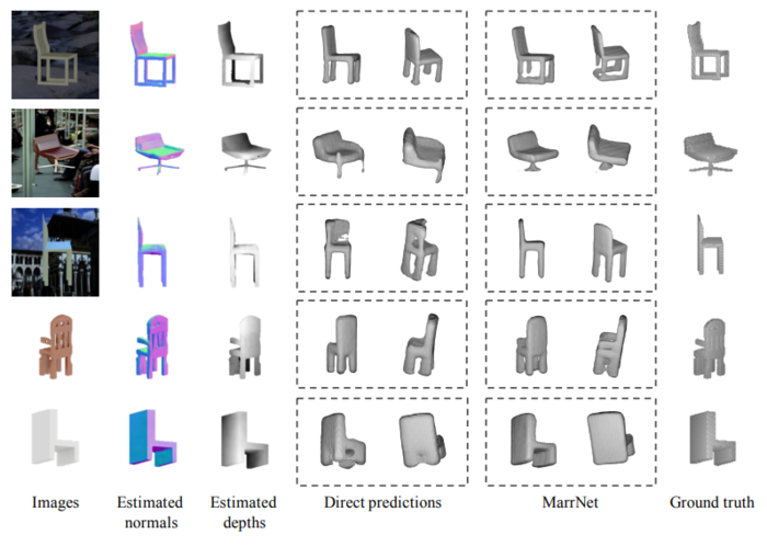
The baseline output is compared to the full framework, and the figure below shows that MarrNet provides model outputs with more details and smoother surfaces than the baseline. The estimated normal and depth images are able to extract intrinsic information about object shape while leaving behind non-essential information such as textures from the original images. Quantitatively, the full model also achieves 0.57 IoU, higher than the direct prediction baseline.

ShapeNet results.

PASCAL 3D+

Rough 3D models are provided from real-life images.

Method

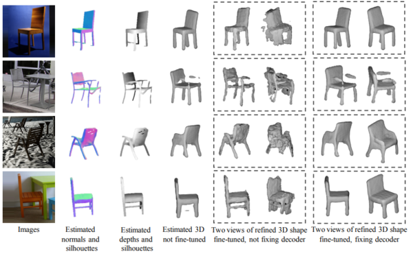
Each module is pre-trained on the ShapeNet dataset, and then fine-tuned on the PASCAL 3D+ dataset. Three variants of the model are tested. The first is trained using ShapeNet data only with no fine-tuning. The second is fine-tuned without fixing the decoder. The third is fine-tuned with a fixed decoder.

Results

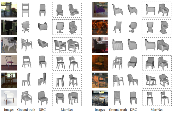
The figure below shows the results of the ablation study. The model trained only on synthetic data provides reasonable estimates. However, fine-tuning without fixing the decoder leads to impossible shapes from certain views. The third model keeps the shape prior, providing more details in the final shape.

Ablation studies using the PASCAL 3D+ dataset.

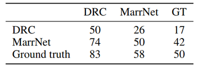
Additional comparisons are made with the state-of-the-art (DRC) on the provided ground truth shapes. MarrNet achieves 0.39 IoU, while DRC achieves 0.34. However, the authors claim that the IoU metric is sub-optimal for three reasons. First, there is no emphasis on details since the metric prefers models that predict mean shapes consistently. Second, all possible scales are searched during the IoU computation, making it less efficient. Third, PASCAL 3D+ only has rough annotations, with only 10 CAD chair models for all images, and computing IoU with these shapes is not very informative. Instead, human studies are conducted and MarrNet reconstructions are preferred 74% of the time over DRC, and 42% of the time to ground truth. This shows how MarrNet produces nice shapes and also highlights the fact that ground truth shapes are not very good.

Human preferences on chairs in PASCAL 3D+ (Xiang et al. 2014). The numbers show the percentage of how often humans prefered the 3D shape from DRC (state-of-the-art), MarrNet, or GT.

Comparison between DRC and MarrNet results.

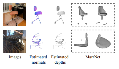
Several failure cases are shown in the figure below. Specifically, the framework does not seem to work well on thin structures.

Failure cases on PASCAL 3D+. The algorithm cannot recover thin structures.

IKEA

This dataset contains images of IKEA furniture, with accurate 3D shape and pose annotations. Objects are often heavily occluded or truncated.

Results

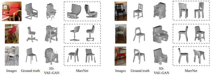
Qualitative results are shown in the figure below. The model is shown to deal with mild occlusions in real life scenarios. Human studes show that MarrNet reconstructions are preferred 61% of the time to 3D-VAE-GAN.

Results on chairs in the IKEA dataset, and comparison with 3D-VAE-GAN.

Other Data

MarrNet is also applied on cars and airplanes. Shown below, smaller details such as the horizontal stabilizer and rear-view mirrors are recovered.

Results on airplanes and cars from the PASCAL 3D+ dataset, and comparison with DRC.

MarrNet is also jointly trained on three object categories, and successfully recovers the shapes of different categories. Results are shown in the figure below.

Results when trained jointly on all three object categories (cars, airplanes, and chairs).

Commentary

Qualitatively, the results look quite impressive. The 2.5D sketch estimation seems to distill the useful information for more realistic looking 3D shape estimation. The disentanglement of 2.5D and 3D estimation steps also allows for easier training and domain adaptation from synthetic data.

As the authors mention, the IoU metric is not very descriptive, and most of the comparisons in this paper are only qualitative, mainly being human preference studies. A better quantitative evaluation metric would greatly help in making an unbiased comparison between different results.

As seen in several of the results, the network does not deal well with objects that have thin structures, which is particularly noticeable with many of the chair arm rests. As well, looking more carefully at some results, it seems that fine-tuning only the 3D encoder does not seem to transfer well to unseen objects, since shape priors have already been learned by the decoder.

Conclusion

The proposed MarrNet employs a novel model to estimate 2.5D sketches for 3D shape reconstruction. The sketches are shown to improve the model’s performance, and make it easy to adapt to images across different domains and categories. Differentiable loss functions are created such that the model can be fine-tuned end-to-end on images without ground truth. The experiments show that the model performs well, and human studies show that the results are preferred over other methods.

Implementation

The following repository provides the source code for the paper. The repository provides the source code as written by the authors: https://github.com/jiajunwu/marrnet

References

1. David Marr. Vision: A computational investigation into the human representation and processing of visual information. W. H. Freeman and Company, 1982.
2. Shubham Tulsiani, Tinghui Zhou, Alexei A Efros, and Jitendra Malik. Multi-view supervision for single-view reconstruction via differentiable ray consistency. In CVPR, 2017.
3. JiajunWu, Chengkai Zhang, Tianfan Xue,William T Freeman, and Joshua B Tenenbaum. Learning a Proba- bilistic Latent Space of Object Shapes via 3D Generative-Adversarial Modeling. In NIPS, 2016b.
4. Wu, J. (n.d.). Jiajunwu/marrnet. Retrieved March 25, 2018, from https://github.com/jiajunwu/marrnet