stat946w18/Tensorized LSTMs

Presented by

Chen, Weishi(Edward)

Introduction

Long Short-Term Memory (LSTM) is a popular approach to boosting the ability of Recurrent Neural Networks to store longer term temporal information. The capacity of an LSTM network can be increased by widening and adding layers (illustrations will be provided later).

However, usually the LSTM model introduces additional parameters, while LSTM with additional layers and wider layers increases the time required for model training and evaluation. As an alternative, the paper <Wider and Deeper, Cheaper and Faster: Tensorized LSTMs for Sequence Learning> has proposed a model based on LSTM call the Tensorized LSTM in which the hidden states are represented by tensors and updated via a cross-layer convolution.

• By increasing the tensor size, the network can be widened efficiently without additional parameters since the parameters are shared across different locations in the tensor
• By delaying the output, the network can be deepened implicitly with little additional runtime since deep computations for each time step are merged into temporal computations of the sequence.

Also, the paper has presented presented experiments conducted on five challenging sequence learning tasks show the potential of the proposed model.

A Quick Introduction to RNN and LSTM

We consider the time-series prediction task of producing a desired output [math]\displaystyle{ y_t }[/math] at each time-step t∈ {1, ..., T} given an observed input sequence [math]\displaystyle{ x1: t = {x_1,x_2, ···, x_t} }[/math], where [math]\displaystyle{ x_t∈R^R }[/math] and [math]\displaystyle{ y_t∈R^S }[/math] are vectors. RNN learns how to use a hidden state vector [math]\displaystyle{ h_t ∈ R^M }[/math] to encapsulate the relevant features of the entire input history x1:t (indicates all inputs from to initial time-step to final step before predication - illustration given below) up to time-step t.

\begin{align} h_{t-1}^{cat} = [x_t, h_{t-1}] \hspace{2cm} (1) \end{align}

Where [math]\displaystyle{ h_{t-1}^{cat} ∈R^{R+M} }[/math] is the concatenation of the current input [math]\displaystyle{ x_t }[/math] and the previous hidden state [math]\displaystyle{ h_{t−1} }[/math], which expands the dimensionality of intermediate information.

The update of the hidden state ht is defined as:

\begin{align} a_{t} =h_{t-1}^{cat} W^h + b^h \hspace{2cm} (2) \end{align}

and

\begin{align} h_t = \Phi(a_t) \hspace{2cm} (3) \end{align}

[math]\displaystyle{ W^h∈R^(R+M)xM }[/math] guarantees each hidden status provided by the previous step is of dimension M. [math]\displaystyle{ a_t ∈R^M }[/math] the hidden activation, and φ(·) the element-wise "tanh" function. Finally, the output [math]\displaystyle{ y_t }[/math] at time-step t is generated by:

\begin{align} y_t = \varphi(h_{t}^{cat} W^y + b^y) \hspace{2cm} (4) \end{align}

where [math]\displaystyle{ W^y∈R^{M×S} }[/math] and [math]\displaystyle{ b^y∈R^S }[/math], and [math]\displaystyle{ \varphi(·) }[/math] can be any differentiable function, notes that the "Phi" is the element-wise function which produces some non-linearity and further generates another hidden status, while the "Curly Phi" is applied to generates the output

Figure 1: Recurrent Neural Network

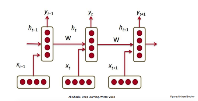
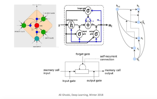
However, one shortfall of RNN is the vanishing/exploding gradients. This shortfall is more significant especially when constructing long-range dependencies models. One alternative is to apply LSTM (Long Short-Term Memories), LSTMs alleviate these problems by employing memory cells to preserve information for longer, and adopting gating mechanisms to modulate the information flow. Since LSTM is successfully in sequence models, it is natural to consider how to increase the complexity of the model to accommodate more complex analytical needs.

Figure 2: LSTM

Structural Measurement of Sequential Model

We can consider the capacity of a network consists of two components: the width (the amount of information handled in parallel) and the depth (the number of computation steps).

A way to widen the LSTM is to increase the number of units in a hidden layer; however, the parameter number scales quadratically with the number of units. To deepen the LSTM, the popular Stacked LSTM (sLSTM) stacks multiple LSTM layers. The drawback of sLSTM, however, is that runtime is proportional to the number of layers and information from the input is potentially lost (due to gradient vanishing/explosion) as it propagates vertically through the layers. This paper introduced a way to both widen and deepen the LSTM whilst keeping the parameter number and runtime largely unchanged. In summary, we make the following contributions:

(a) Tensorize RNN hidden state vectors into higher-dimensional tensors, to enable more flexible parameter sharing and can be widened more efficiently without additional parameters.

(b) Based on (a), merge RNN deep computations into its temporal computations so that the network can be deepened with little additional runtime, resulting in a Tensorized RNN (tRNN).

(c) We extend the tRNN to an LSTM, namely the Tensorized LSTM (tLSTM), which integrates a novel memory cell convolution to help to prevent the vanishing/exploding gradients.

Method

Go through the methodology.

Part 1: Tensorize RNN hidden State vectors

Definition: Tensorization is defined as the transformation or mapping of lower-order data to higher-order data. For example, the low-order data can be a vector, and the tensorized result is a matrix, a third-order tensor or a higher-order tensor. The ‘low-order’ data can also be a matrix or a third-order tensor, for example. In the latter case, tensorization can take place along one or multiple modes.

Figure 3: Vector Third-order tensorization of a vector

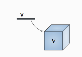
Optimization Methodology Part 1: It can be seen that in an RNN, the parameter number scales quadratically with the size of the hidden state. A popular way to limit the parameter number when widening the network is to organize parameters as higher-dimensional tensors which can be factorized into lower-rank sub-tensors that contain significantly fewer elements, which is is known as tensor factorization.

Optimization Methodology Part 2: Another common way to reduce the parameter number is to share a small set of parameters across different locations in the hidden state, similar to Convolutional Neural Networks (CNNs).

Effects: This widens the network since the hidden state vectors are in fact broadcast to interact with the tensorized parameters.

We adopt parameter sharing to cutdown the parameter number for RNNs, since compared with factorization, it has the following advantages:

(i) Scalability, the number of shared parameters can be set independent of the hidden state size

(ii) Separability, the information flow can be carefully managed by controlling the receptive field, allowing one to shift RNN deep computations to the temporal domain

We also explicitly tensorize the RNN hidden state vectors, since compared with vectors, tensors have a better:

(i) Flexibility, one can specify which dimensions to share parameters and then can just increase the size of those dimensions without introducing additional parameters

(ii) Efficiency, with higher-dimensional tensors, the network can be widened faster w.r.t. its depth when fixing the parameter number (explained later).

Illustration: For ease of exposition, we first consider 2D tensors (matrices): we tensorize the hidden state [math]\displaystyle{ h_t∈R^{M} }[/math] to become [math]\displaystyle{ Ht∈R^{P×M} }[/math], where P is the tensor size, and M the channel size. We locally-connect the first dimension of [math]\displaystyle{ H_t }[/math] (which is P - the tensor size) in order to share parameters, and fully-connect the second dimension of [math]\displaystyle{ H_t }[/math] (which is M - the channel size) to allow global interactions. This is analogous to the CNN which fully-connects one dimension (e.g., the RGB channel for input images) to globally fuse different feature planes. Also, if one compares [math]\displaystyle{ H_t }[/math] to the hidden state of a Stacked RNN (sRNN) (see Figure Blow).

Figure 4: Stacked RNN

Figure 4: Stacked RNN

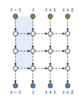
Then P is akin to the number of stacked hidden layers (vertical length in the graph), and M the size of each hidden layer (each white node in the graph). We start to describe our model based on 2D tensors, and finally show how to strengthen the model with higher-dimensional tensors.

Part 2: Merging Deep Computations

Since an RNN is already deep in its temporal direction, we can deepen an input-to-output computation by associating the input [math]\displaystyle{ x_t }[/math] with a (delayed) future output. In doing this, we need to ensure that the output [math]\displaystyle{ y_t }[/math] is separable, i.e., not influenced by any future input [math]\displaystyle{ x_{t^{'}} }[/math] [math]\displaystyle{ (t^{'}\gt t) }[/math]. Thus, we concatenate the projection of [math]\displaystyle{ x_t }[/math] to the top of the previous hidden state [math]\displaystyle{ H_{t−1} }[/math], then gradually shift the input information down when the temporal computation proceeds, and finally generate [math]\displaystyle{ y_t }[/math] from the bottom of [math]\displaystyle{ H_{t+L−1} }[/math], where L−1 is the number of delayed time-steps for computations of depth L.

An example with L= 3 is shown in Figure.

Figure 5: skewed sRNN

Figure 5: skewed sRNN

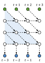
This is in fact a skewed sRNN (or tRNN without feedback). However, the method does not need to change the network structure and also allows different kinds of interactions as long as the output is separable; for example, one can increase the local connections and use feedback (shown in figure below), which can be beneficial for sRNNs (or tRNN).

Figure 5: skewed sRNN with F

Figure 5: skewed sRNN with F

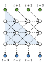
In order to share parameters, we update [math]\displaystyle{ H_t }[/math] using a convolution with a learnable kernel. In this manner we increase the complexity of the input-to-output mapping (by delaying outputs) and limit parameter growth (by sharing transition parameters using convolutions).

To examine the resulting model mathematically, let [math]\displaystyle{ H^{cat}_{t−1}∈R^{(P+1)×M} }[/math] be the concatenated hidden state, and [math]\displaystyle{ p∈Z_+ }[/math] the location at a tensor. The channel vector [math]\displaystyle{ h^{cat}_{t−1, p }∈R^M }[/math] at location p of [math]\displaystyle{ H^{cat}_{t−1} }[/math] (the p-th channel of H) is defined as:

\begin{align} h^{cat}_{t-1, p} = x_t W^x + b^x \hspace{1cm} if p = 1 \hspace{1cm} (5) \end{align}

\begin{align} h^{cat}_{t-1, p} = h_{t-1, p-1} \hspace{1cm} if p > 1 \hspace{1cm} (6) \end{align}

where [math]\displaystyle{ W^x ∈ R^{R×M} }[/math] and [math]\displaystyle{ b^x ∈ R^M }[/math] (recall the dimension of input x is R). Then, the update of tensor [math]\displaystyle{ H_t }[/math] is implemented via a convolution:

\begin{align} A_t = H^{cat}_{t-1} \circledast \{W^h, b^h \} \hspace{2cm} (7) \end{align}

\begin{align} H_t = \Phi{A_t} \hspace{2cm} (8) \end{align}

where [math]\displaystyle{ W^h∈R^{K×M^i×M^o} }[/math] is the kernel weight of size K, with [math]\displaystyle{ M^i =M }[/math] input channels and [math]\displaystyle{ M^o =M }[/math] output channels, [math]\displaystyle{ b^h ∈ R^{M^o} }[/math] is the kernel bias, [math]\displaystyle{ A_t ∈ R^{P×M^o} }[/math] is the hidden activation, and [math]\displaystyle{ \circledast }[/math] is the convolution operator. Since the kernel convolves across different hidden layers, we call it the cross-layer convolution. The kernel enables interaction, both bottom-up and top-down across layers. Finally, we generate [math]\displaystyle{ y_t }[/math] from the channel vector [math]\displaystyle{ h_{t+L−1,P}∈R^M }[/math] which is located at the bottom of [math]\displaystyle{ H_{t+L−1} }[/math]:

\begin{align} y_t = \varphi(h_{t+L−1}, _PW^y + b^y) \hspace{2cm} (9) \end{align}

Where [math]\displaystyle{ W^y ∈R^{M×S} }[/math] and [math]\displaystyle{ b^y ∈R^S }[/math]. To guarantee that the receptive field of [math]\displaystyle{ y_t }[/math] only covers the current and previous inputs x1:t. (Check the Skewed sRNN again below):

Figure 5: skewed sRNN with F

Figure 5: skewed sRNN with F

Quick Summary of Set of Parameters

1. [math]\displaystyle{ W^x }[/math] and [math]\displaystyle{ b_x }[/math] connect input to the first hidden node

2. [math]\displaystyle{ W^h }[/math] and [math]\displaystyle{ b_h }[/math] convolute between layers

3. [math]\displaystyle{ W^y }[/math] and [math]\displaystyle{ b_y }[/math] produce output of each stages

Part 3: Extending to LSTMs

Similar to standard RNN, to allow the tRNN (skewed sRNN) to capture long-range temporal dependencies, one can straightforwardly extend it to a tLSTM by replacing the tRNN tensors:

\begin{align} [A^g_t, A^i_t, A^f_t, A^o_t] = H^{cat}_{t-1} \circledast \{W^h, b^h \} \hspace{2cm} (10) \end{align}

\begin{align} [G_t, I_t, F_t, O_t]= [\Phi{(A^g_t)}, σ(A^i_t), σ(A^f_t), σ(A^o_t)] \hspace{2cm} (11) \end{align}

Which are pretty similar to tRNN case, the main differences can be observes for memory cells of tLSTM (Ct):

\begin{align} C_t= G_t \odot I_t + C_{t-1} \odot F_t \hspace{2cm} (12) \end{align}

\begin{align} H_t= \Phi{(C_t )} \odot O_t \hspace{2cm} (13) \end{align}

Summary of the terms:

1. [math]\displaystyle{ G_t }[/math]: Activation of new content

2. [math]\displaystyle{ I_t }[/math]: Input gate

3. [math]\displaystyle{ F_t }[/math]: Forget gate

4. [math]\displaystyle{ O_t }[/math]: Output gate

Then, see graph below for illustration:

Figure 5: tLSTM wo MC

Figure 5: tLSTM wo MC

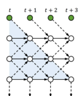
To further evolve tLSTM, we invoke the Memory Cell Convolution to capture long-range dependencies from multiple directions, we additionally introduce a novel memory cell convolution, by which the memory cells can have a larger receptive field (figure provided below).

Figure 5: tLSTM w MC

Figure 5: tLSTM w MC

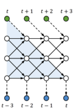
One can also dynamically generate this convolution kernel so that it is both time - and location-dependent, allowing for flexible control over long-range dependencies from different directions. Mathematically, it can be represented in with the following formulas:

\begin{align} [A^g_t, A^i_t, A^f_t, A^o_t, A^q_t] = H^{cat}_{t-1} \circledast \{W^h, b^h \} \hspace{2cm} (14) \end{align}

\begin{align} [G_t, I_t, F_t, O_t, Q_t]= [\Phi{(A^g_t)}, σ(A^i_t), σ(A^f_t), σ(A^o_t), ς(A^q_t)] \hspace{2cm} (15) \end{align}

\begin{align} W_t^c(p) = reshape(q_{t,p}, [K, 1, 1]) \hspace{2cm} (16) \end{align}

\begin{align} C_{t-1}^{conv}= C_{t-1} \circledast W_t^c(p) \hspace{2cm} (17) \end{align}

\begin{align} C_t= G_t \odot I_t + C_{t-1}^{conv} \odot F_t \hspace{2cm} (18) \end{align}

\begin{align} H_t= \Phi{(C_t )} \odot O_t \hspace{2cm} (19) \end{align}

where the kernel [math]\displaystyle{ {W^h, b^h} }[/math] has additional <K> output channels to generate the activation [math]\displaystyle{ A^q_t ∈ R^{P×\lt K\gt } for the dynamic kernel bank \lt math\gt Q_t∈R^{Px\lt K\gt } }[/math], [math]\displaystyle{ q_{t,p}∈R^\lt K\gt }[/math] is the vectorized adaptive kernel at the location p of [math]\displaystyle{ Q_t }[/math], and [math]\displaystyle{ W^c_t(p) ∈ R^{K×1×1} is the dynamic kernel of size K with a single input/output channel, which is reshaped from qt,p. Note the paper also employed a softmax function ς(·) to normalize the channel dimension of \lt math\gt Q_t }[/math].