Learning Combinatorial Optimzation

Learning Combinatorial Optimization Algorithms Over Graphs

Group Members

Abhi (Introduction),

Alvin (actual paper)

Pranav (actual paper),

Daniel (Conclusion: performance, adv, disadv, criticism)

1. Introduction and Problem Motivation

The current approach to tackling NP-hard combinatorial optimization problems are good heuristics or approximation algorithms. While these approaches have been adequate, it requires specific domain-knowledge behind each individual problem or additional trial-and-error in determining the tradeoff being finding an accurate or efficient heuristics function. However, if these problems are repeated solved, differing only in data values, perhaps we could apply learning on heuristics functions such that we automate this tedious task.

The authors of this paper present an approach that learns heuristics functions through the combination of reinforcement learning and graph embedding. With reinforcement learning the policy learns a greedy approach in incrementally constructing a solution. To determine the greedy action, the current state of the problem is taken as input to a graph embedding network from which an action will be given by its output.

2. Prerequisite Knowledge and Example Problems

a) Graph Theory

Graph Theory is the study of mathematical structures used to model relation between objects. All graphs are made up of a series of vertices (points), edges (lines). These problems have a common notation of: G=(V,E,w)

Where G is the Graph, V are the vertices, E is the set of edges, and w is the set of weights for the edges

The three main problems which the paper proposes a solution for are:

Minimum Vertex Cover: Given a ‘graph’ G. If there exists a set of vertices (S) so that every edge touches at least 1 point in S, then we can say that every element in S is a vertex cover. In a minimum vertex cover problem, the goal is to find the minimum possible size of S. A quick example of this is below, you can see that when those 2 red vertices are ticked, every single edge is now touching a red vertex.

Maximum Cut: Given a G. A cut is the splitting of a graph into 2 parts (S and T). In a Max cut problem, the goal is to cut the graph in such a way that the number of edges that are touching both vertices of S and T at the same time is maximized. A quick example of this is below, you can see that when those 2 pink vertices are ticked, the number of edges that touch a vertex in S, and T is maximized, and the maximum value for this solution is 8.

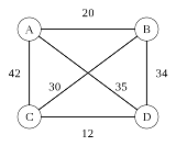
Travelling Salesman Problem: In the travelling Salesman problem, if you have a list of cities and their distance between each other, how can you navigate through each of the cities so that you'll visit every city, and return back to the origin as quick as possible. This problem can be represented in a Graph, where each of the vertices (V) represents the cities, and each of the edges (E) represents the distance between each of the cities. A small example is shown below.

b) Reinforcement Learning

The core concept of Reinforcement Learning is to consider a partially observable Markov Decision Process, and a A Markov decision process is a 5-tuple [math]\displaystyle{ (S,A,P_\cdot(\cdot,\cdot),R_\cdot(\cdot,\cdot),\gamma) }[/math], where

• [math]\displaystyle{ S }[/math] is a finite set of states (they do not have to be, but for the purpose of this paper, we assume for it to be),
• [math]\displaystyle{ A }[/math] is a finite set of actions (generally only feasible actions) (alternatively, [math]\displaystyle{ A_s }[/math] is the finite set of actions available from state [math]\displaystyle{ s }[/math]),
• [math]\displaystyle{ P_a(s,s') = \Pr(s_{t+1}=s' \mid s_t = s, a_t=a) }[/math] is the probability that action [math]\displaystyle{ a }[/math] in state [math]\displaystyle{ s }[/math] at time [math]\displaystyle{ t }[/math] will lead to state [math]\displaystyle{ s' }[/math] at time [math]\displaystyle{ t+1 }[/math],
• [math]\displaystyle{ R_a(s,s') }[/math] is the immediate reward (or expected immediate reward) received after transitioning from state [math]\displaystyle{ s }[/math] to state [math]\displaystyle{ s' }[/math], due to action [math]\displaystyle{ a }[/math], furthermore, it is between two consecutive time periods
• [math]\displaystyle{ \gamma \in [0,1] }[/math] is the discount factor, which represents the difference in importance between future rewards and present rewards.

In Reinforcement Learning, the rules are generally stochastic, which means that we associate a probability with choosing an action as opposed to deterministic choice of an action. Some other talks have elucidated about this, however, in detail, the idea is that, to maintain exploration-exploitation tradeoffs it's a good idea to have a list of probabilities as opposed to random values.

3. Representation

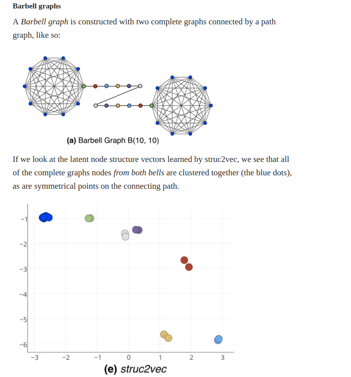
The choice of representation for the graph, as mentioned above, is known as struct2vec. The intuitive idea of this is very similar to word2vec which is a very popular model for encoding words into a low dimensional space. We begin with explaining [math]\displaystyle{ \hat{Q} }[/math] which can be thought of summarizing the state of a graph at a given point in time. In the Reinforcement Learning literature, [math]\displaystyle{ \hat{Q} }[/math] is often thought of a measure of quality, in this case, it can be thought of that way too, where the quality of the graph represents how much cost we have avoided.

But representing complex structures is extremely hard, in fact one may always argue that there is some property of the graph that the algorithm has failed to capture, we will elaborate on this in the criticisms of the paper.

Struct2Vec aims to gather information about the graph topology which could represent how to traverse it using the greedy algorithm. This is a claim that the paper makes without any justification, they claim in the struct2vec paper that measuring similarity in the degrees in vertices represents structural relationships between the nodes. However, it is not impossible to think of a mathematical or intuitive counterexample to this problem, especially when it comes to the TSP/maxcut.

[math]\displaystyle{ \mu_v^{t + 1} \leftarrow \mathcal{F}(x_v, \{\mu_u\}_{u \in \mathcal{N}(v)}, \{w(v, u)\}_{u \in \mathcal{N}(v)}; \Theta) }[/math]

Where:

1. [math]\displaystyle{ \mathcal{N}(v) - \text{Neighborhood of v} }[/math]

2. [math]\displaystyle{ \mathcal{F} - \text{Non Linear Mapping} }[/math]

3. [math]\displaystyle{ x_v - \text{Current features of the nodes} }[/math]

This formula is explicitly given by: [math]\displaystyle{ \mu_v^{t + 1} \leftarrow \text{relu}(\theta_1 x_v + \theta_2 \sum_{u \in \mathcal{N}(v)} \mu_u^{t} + \theta_3 \sum_{u \in \mathcal{N}(v)} relu(\theta_4 \cdot w(v, u)) }[/math]. There are a few interesting facts about this formula, one of them is: the fact that they've used summations, which makes the algorithm order invariant, possibly because they believe the order of the nodes is not really relevant, however, this is fairly contradictory to the baseline they compare against (which is location dependent/order dependent). Also, one might ask the question that, what if the topology allows for updates to be dependent on future updates. This is why it happens over several iterations (the paper presents 4 as a decent number). It does make sense that as we increase the value of [math]\displaystyle{ T }[/math], we will see that nodes are dependent on other nodes they are very far away from.

We also highlight the dimensions of the parameters: [math]\displaystyle{ \theta_1, \theta_4 \in \mathbb{R}^p, \theta_2, \theta_3 \in \mathbb{R}^{p \times p} }[/math]. Now, with this new information about our graphs, we must compute our estimated value function for pursuing a particular action.

[math]\displaystyle{ \hat{Q}(h(S), v;\Theta) = \theta_5^{T} relu([\theta_6 \sum_{u \in V} \mu_u^{(T)}, \theta_7 \mu_v^{(T)}]) }[/math].

Where, [math]\displaystyle{ \theta_5 \in \mathbb{R}^{2p}, \theta_6, \theta_7 \in \mathbb{R}^{p \times p} }[/math].

Finally, [math]\displaystyle{ \Theta = \{\theta_i\}_{i=1}^{7} }[/math]

4. Training

Formulating of Reinforcement learning:

1. States - S is the state of the graph at a given time which is obtained through an action

2. Transition - Transitioning to another node; Tag the node that was last used with feature x = 1

3. Actions - An action is a node of the graph that isn't part of the sequence of actions. Actions are p-dimensional nodes.

4. Rewards - Reward function is defined as change in cost after action and movement.

More specifically,

[math]\displaystyle{ r(S,v) = c(h(S'),G) - c(h(S),G); }[/math]

This represents change in cost evaluated from previous state to new state

For the three optimization problems: MVC, MAXCUT, TSP; we have different formulations of reinforcement learning (States, Transitions, Actions, Rewards)

[math]\displaystyle{ \text{Learning Algorithm:} }[/math]

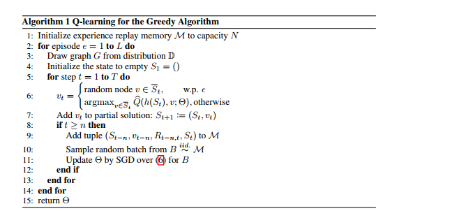
To perform learning of the parameters, application of n-step Q learning and fitted Q-iteration is used.

Stepped Q-learning: This updates the function's parameters at each step by performing a gradient step to minimize the squared loss of the function.

[math]\displaystyle{ (y- Q(h(S_t),v_t; \theta))^2 }[/math] where

[math]\displaystyle{ y = (\gamma max_v Q(h(S_t+1),v';\theta) + r(S_t,v_t) }[/math].

Generalizing to n-step Q learning, it addresses the issue of delayed rewards, where an immediate valuation of rewards may not be optimal. With this instance, one- step updating of the parameters may not be optimal.

Fitted Q-learning: Is a faster learning convergence when used on top of a neural network. In contrast to updating Q function sample by sample, it updates function with batches of samples from data set instead of singular samples.

5. Results and Criticisms

The paper proposes a solution that uses a combination of reinforcement learning and graph embedding to improve current methods of solving graph optimization problems. However, the graph embedding network the authors use is called struct2vec (S2V). S2V takes a graph as input and converts the properties of the nodes in the graph as features. This entails picking a fixed output dimension which may or may not compromise on the expressibility of the node, i.e. we may lose information by arbitrarily choosing an output dimension. In particular, knowing a node’s neighbourhood is useful in problems such as Minimum Vertex Cover or Maximum Cut, however it may not be as useful in problems such as Traveling Salesman Problem.

Another criticism for the paper is the choice of algorithms to compare against. While it is completely up to the authors to choose what they compare their algorithms against, it does seem strange to compare their Reinforcement Learning algorithm to some of the worse insertion heuristics for the TSP. In particular, there are a couple of insertion heuristics that underperform, i.e., choose far below suboptimal tours. It would be very helpful to indicate this to the audience reading the paper. Similarly, for pointer networks being the benchmark.

6. Conclusions

TODO: Add the tables from the paper for comparisons The machine learning framework the authors propose is a solution to NP-hard graph optimization problems that have a large amount of instances that need to be computed. Where the problem structure remains largely the same except for specific data values. Such cases are common in the industry where large tech companies have to process millions of requests per second and can afford to invest in expensive pre-computation if it speeds up real-time individual requests. Through their experiments and performance results the paper has shown that their solution could potentially lead to faster development and increased runtime efficiency of algorithms for graph problems.

7. Source

Hanjun Dai, Elias B. Khalil, Yuyu Zhang, Bistra Dilkina, Le Song. Learning Combinatorial Optimization Algorithms over Graphs. In Neural Information Processing Systems, 2017

https://blog.acolyer.org/2017/09/15/struc2vec-learning-node-representations-from-structural-identity/