Dynamic Routing Between Capsules

Group Member

Siqi Chen, Weifeng Liang, Yi Shan, Yao Xiao, Yuliang Xu, Jiajia Yin, Jianxing Zhang

Motivation

Why CNN doesn't always work?

In CNN, there's always at least one pooling stage. If we take max-pooling method as an example, the idea is to take the maximum value from a neighborhood, so that when the information is passed to the next layer, we can adjust the dimensions whatever ways we want, and in most cases, we want to reduce the number of dimensions because we always want to save computations. The reason behind this kind of pooling method is based on the correlations within adjacent area. There’re two examples: one (Netflix users’ preferences )is from the example in Ali’s Youtube videos, the other is about the observation of pictures. We will illustrate these two examples in class. So we can see, the problem with local pooling method is that, it only passes the local patterns into the next layer. That is to say, if our original data set doesn't have the good property of neighborhood resemblance, or is simply rearranged by different components, our machine can no longer recognize the picture or make predictions. Although pooling methods save lots of computational power, but it leads the whole CNN methods (i.e. the machine) towards recognizing the local patterns in an image to make judgement instead of looking at the whole picture. Our goal is to train the machine do things in a way, if not beyond human, resembles human thinking.

"They do not encode the position and orientation of the object into their predictions. They completely lose all their internal data about the pose and the orientation of the object and they route all the information to the same neurons that may not be able to deal with this kind of information.

A CNN makes predictions by looking at an image and then checking to see if certain components are present in that image or not. If they are, then it classifies that image accordingly.

In a CNN, all low-level details are sent to all the higher level neurons. These neurons then perform further convolutions to check whether certain features are present. This is done by striding the receptive field and then replicating the knowledge across all the different neurons

According to Professor Hinton, if a lower level neuron has identified an ear, it then makes sense to send this information to a higher level neuron that deals with identifying faces and not to a neuron that identifies chairs. If the higher level face neuron gets a lot of information that contains both the position and the degree of certainty from lower level neurons of the presence of a nose, two eyes and an ear, then the face neuron can identify it as a face.

His solution is to have capsules, or a group of neurons, in lower layers to identify certain patterns. These capsules would then output a high-dimensional vector that contains information about the probability of the position of a pattern and its pose. These values would then be fed to the higher-level capsules that take multiple inputs from many lower-level capsules."

Reference: https://www.quora.com/What-are-some-of-the-limitations-or-drawbacks-of-Convolutional-Neural-Networks

Moreover, there are two more examples which can show the defect of CNN.

The first one is "One pixel attack". Look at the following graph:

So, how to train the machine to look at the whole picture?

In this paper, Professor Geoffrey Hinton gave a solution—using a group of neurons as a capsule to pass the information of orientation and pose.

Introduction to Capsules and Dynamic Routing

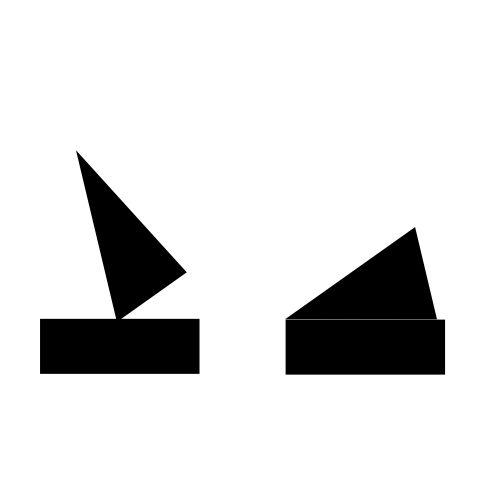
In the following section, we will use a example to classify images of house and boat, both of which are constructed using rectangles and triangles as shown below:

Fig 1.

Introduction to Capsules

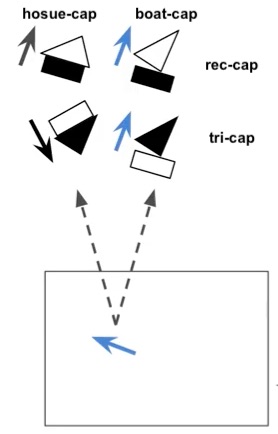
First, let's start with the definition of Capsule. Capsule is a group of neurons that tries to predict the presence and the instantiation parameter of a particular object at the given location. The length of the activity vector of a capsule represent the probability that the object exists, and the orientation of the activity vector represents the instantiation parameters. In the figure below, there are 50 arrows in the left square, and each of them is a capsule. The blue arrows are predicting triangles, and the black ones are predicting the rectangle. In this example, the orientation of the arrows represents the rotation of the shapes. But in reality, the activity vector may have much more dimensions.

Fig 2.

Usually multiple Convolutional Layers are applied to implement capsules, which outputs an array containing feature maps. Then the array is reshaped to get a set of vectors for each location. At the same time, we also need to squash the vectors by [math]\displaystyle{ Squash(u) = \frac{||u||^2}{1+||u||^2} \frac{u}{||u||} }[/math], which preserves the direction of the vector but rescales the range to [0, 1]. We want this range because the length need to represent the probability of the existence of the object.

In the example above, if we rotate the ship, the errors will change their pointing direction correspondingly as well, since they always detect the orientation of the object. This is called [math]\displaystyle{ Equivariance }[/math]. This is an important feature that is not captured by convolutional net. The key difference between capsule and neural network architectures is that others add layers after a layer, but capsule nests a layer inside another layer.

Prediction and Routing

In the above boat and house example, we have two capsules to detect rectangle and triangle. The left part of Figure 2 shows the result from the primary capsule layer. The prediction contains two parts: probability of existence of certain element and the direction. Suppose they will be feed into 2 capsules in the next layer: house-capsule and boat-capsule.

Assume that the rectangle capsule detect a rectangle rotated by 30 degrees, this feed into the next layer will result into house-capsule detecting a house rotated by 30 degrees. Similar for boat-capsule, where a boat rotated by 30 degrees will be detected in the next layer. Mathematically speaking, this can be written as: [math]\displaystyle{ \hat{u}_{ij} = W_{ij} u_i }[/math] where [math]\displaystyle{ u_i }[/math] is the own activation function of this capsule and [math]\displaystyle{ W_{ij} }[/math] is a transformation matrix being developed during training process.

Then look at the prediction from triangle capsule, which provides a different result in house-capsule and boat-capsule.

Fig 2.

Now we have four outputs in total, and we can see that the prediction in boat-capsule strongly agree to each other, which means we can reach the conclusion that the rectangle and triangle are parts of a boat; therefore, they should be routed to the boat-capsule. There is no need to send the output from primary capsule to any other capsules in the next layer, since this action will only add noise. This is the procedure called routing by agreement. Since only necessary outputs will be directed to the next layer, clearer signal will be received, and more accurate result will be produced. To implement routing by agreement, a clustering technique will be used and introduced in the next section.

Clustering and Updating

Fig 3.

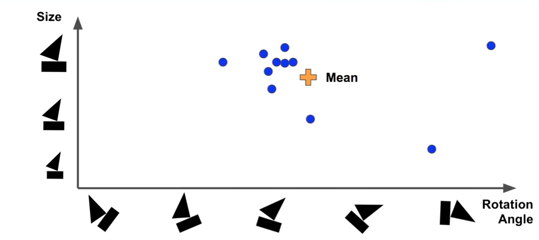
Suppose we represent capsules in the above graph, with x-axis representing rotation angle of the boat and y-axie representing the size. After find out the mean of data, we need to measure the distance between mean and prediction points on the graph by applying Euclidean distance or scalar product. The purpose of this step is to understand how much each prediction vector agrees with the mean, so that the weights of predicted vector can be output and updated. If the prediction matches mean well (i.e. the distance is small), more weights will be assigned to it. After getting the new weights, a weighted-mean will be computed, and it will be used to compute the distance again, and updated iteratively until reaches a steady state.

Mathematically speaking, the procedure starts with 0 weights for all prediction initially. Round1:

 bij = 0 for all i and j
 ci = softmax(bi)
 sj = weighted sum of predictions of each capsule in the next layer  
 vj = squash(sj), which will be the actual outputs of the next layers

After round1, we will update all [math]\displaystyle{ b_{ij} }[/math] as: [math]\displaystyle{ b_{ij} += \hat{u}_j * v_{ji} }[/math], then perform the next steps iteratively.