Do Deep Neural Networks Suffer from Crowding: Difference between revisions
No edit summary |
No edit summary |
||
| Line 26: | Line 26: | ||
==Eccentricity-dependent Model== | ==Eccentricity-dependent Model== | ||
As per Poggio et al. in [18],receptive fields increase in size with eccentricity. The eccentricity-dependent model computes an invariant representation by sampling the inverted pyramid at a discrete set of scales with the same number of filters at each scale. At larger scales, the receptive fields of the filters are also larger to cover a larger image area, see Fig 3(a). Thus, the model constructs a multi-scale representation of the input, where smaller sections (crops) of the image are sampled densely at a high resolution, and larger sections (crops) are sampled with at a lower resolution, with each scale represented using the same number of pixels, as shown in Fig . Each scale is treated as an input channel to the network and then processed by convolutional filters, the weights of which are shared also across scales as well as space. Because of the downsampling of the input image, this is equivalent to having receptive fields of varying sizes. These shared parameters also allow the model to learn a scale invariant representation of the image. | As per Poggio et al. in [18],receptive fields increase in size with eccentricity. The eccentricity-dependent model computes an invariant representation by sampling the inverted pyramid at a discrete set of scales with the same number of filters at each scale. At larger scales, the receptive fields of the filters are also larger to cover a larger image area, see Fig 3(a). Thus, the model constructs a multi-scale representation of the input, where smaller sections (crops) of the image are sampled densely at a high resolution, and larger sections (crops) are sampled with at a lower resolution, with each scale represented using the same number of pixels, as shown in Fig . Each scale is treated as an input channel to the network and then processed by convolutional filters, the weights of which are shared also across scales as well as space. Because of the downsampling of the input image, this is equivalent to having receptive fields of varying sizes. These shared parameters also allow the model to learn a scale invariant representation of the image. | ||
[[File:EDM.png| | [[File:EDM.png|2000x450px|center]] | ||
Scale pooling reduces the number of scales by taking the maximum value of corresponding locations in the feature maps across multiple scales. We set the spatial pooling constant using At end pooling, as described above. The type of scale pooling is indicated by writing the number of scales remaining in each layer, e.g. 11-1-1-1-1. The three configurations tested for scale pooling are (1) at the beginning, in which all the different scales are pooled together after the first layer, 11-1-1-1-1 (2) progressively, 11-7-5-3-1 and (3) at the end, 11-11-11-11-1, in which all 11 scales are pooled together at the last layer. | Scale pooling reduces the number of scales by taking the maximum value of corresponding locations in the feature maps across multiple scales. We set the spatial pooling constant using At end pooling, as described above. The type of scale pooling is indicated by writing the number of scales remaining in each layer, e.g. 11-1-1-1-1. The three configurations tested for scale pooling are (1) at the beginning, in which all the different scales are pooled together after the first layer, 11-1-1-1-1 (2) progressively, 11-7-5-3-1 and (3) at the end, 11-11-11-11-1, in which all 11 scales are pooled together at the last layer. | ||
| Line 41: | Line 41: | ||
==DNNs trained with Target and Flankers== | ==DNNs trained with Target and Flankers== | ||
This is a constant spacing training setup where identical flankers are placed at a distance of 120 pixels either side of the target(xax) with the targte having translational variance. THe tests are evaluated on (i) DCNN with at the end pooling, and (ii) eccentricity-dependent model with 11-11-11-11-1 scale pooling, at the end spatial pooling and contrast normalization. The test data has different flanker configurations as described above. | This is a constant spacing training setup where identical flankers are placed at a distance of 120 pixels either side of the target(xax) with the targte having translational variance. THe tests are evaluated on (i) DCNN with at the end pooling, and (ii) eccentricity-dependent model with 11-11-11-11-1 scale pooling, at the end spatial pooling and contrast normalization. The test data has different flanker configurations as described above. | ||
[[File:result1.png|x450px|center]] | |||
===Observations=== | ===Observations=== | ||
- With the flanker configuration same as the training one, models are better at recognizing objects in clutter rather than isolated objects for all image locations | |||
-If the target-flanker spacing is changed, then models perform worse | |||
-the eccentricity model is much better at recognizing objects in isolation than the DCNN because the multi-scale crops divide the image into discrete regions, letting the model learn from image parts as well as the whole image | |||
-Only the eccentricity-dependent model is robust to different flanker configurations not included in training, when the target is centered. | |||
==DNNs trained with Images with the Target in Isolation== | |||
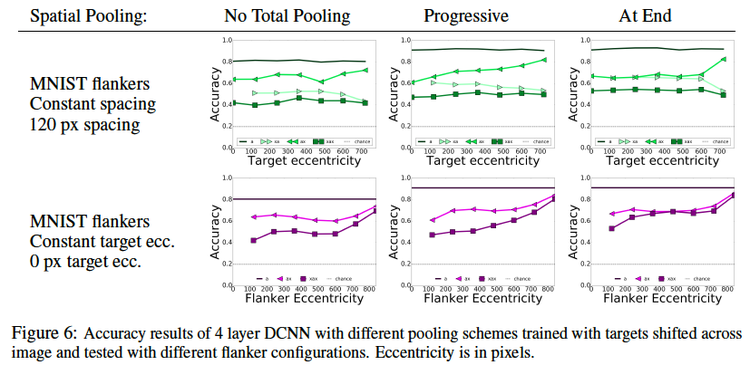
[[File:result2.png|750x400px|center]] | |||
===Eccentric Model=== | |||
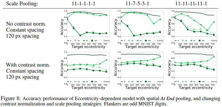
[[File:result3.png|750x400px|center]] | |||
=Conclusions= | =Conclusions= | ||
We often think that just training the network with data similar to the test data would achieve good results in a general scenario too but thats not the case as we trained the model with flankers and it did not give us the ideal results for the target obects. | We often think that just training the network with data similar to the test data would achieve good results in a general scenario too but thats not the case as we trained the model with flankers and it did not give us the ideal results for the target obects. | ||
*'''Flanker Configuration''': When models are trained with images of objects in isolation, adding flankers harms recognition. Adding two flankers is the same or worse than adding just one and the smaller the spacing between flanker and target, the more crowding occurs. These is because the pooling operation merges nearby responses, such as the target and flankers if they are close. | |||
*'''Similarity between target and flanker''': Flankers more similar to targets cause more crowding, because of the selectivity property of the learned DNN filters. | |||
*'''Dependence on target location and contrast normalization''': In DCNNs and eccentricitydependent models with contrast normalization, recognition accuracy is the same across all eccentricities. In eccentricity-dependent networks without contrast normalization, recognition does not decrease despite presence of clutter when the target is at the center of the image. | |||
*'''Effect of pooling''': adding pooling leads to better recognition accuracy of the models. Yet, in the eccentricity model, pooling across the scales too early in the hierarchy leads to lower accuracy. | |||
Revision as of 01:07, 20 March 2018
Still working on this.
Introduction
Ever since the evolution of Deep Networks, there has been tremendous amount of research and effort that has been put into making machines capable of recognizing objects the same way as humans do. Humans can recognize objects in a way that is invariant to scale, translation, and clutter. Crowding is another visual effect suffered by humans, in which an object that can be recognized in isolation can no longer be recognized when other objects, called flankers, are placed close to it and this is a very common real-life experience. This paper focuses on studying the impact of crowding on Deep Neural Networks (DNNs) by adding clutter to the images and then analyzing which models and settings suffer less from such effects.
The paper investigates two types of DNNs for crowding: traditional deep convolutional neural networks(DCNN) and a multi-scale eccentricity-dependent model which is an extension of the DCNNs and inspired by the retina where the receptive field size of the convolutional filters in the model grows with increasing distance from the center of the image, called the eccentricity and will be explained below. The authors focus on the dependence of crowding on image factors, such as flanker configuration, target-flanker similarity, target eccentricity and premature pooling in particular.
Models
Deep Convolutional Neural Networks
The DCNN is a basic architecture with 3 convolutional layers, spatial 3x3 max-pooling with varying strides and a fully connected layer for classification as shown in the below figure.
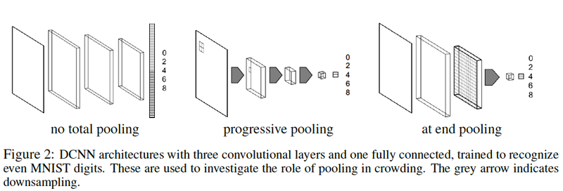
The network is fed with images resized to 60x60, with minibatches of 128 images, 32 feature channels for all convolutional layers, and convolutional filters of size 5x5 and stride 1.
As highlighted earlier, the effect of pooling is into main consideration and hence three different configurations have been investigated as below:
1. No total pooling Feature maps sizes decrease only due to boundary effects, as the 3x3 max pooling has stride 1. The square feature maps sizes after each pool layer are 60-54-48-42.
2. Progressive pooling 3x3 pooling with a stride of 2 halves the square size of the feature maps, until we pool over what remains in the final layer, getting rid of any spatial information before the fully connected layer. (60-27-11-1).
3. At end pooling Same as no total pooling, but before the fully connected layer, max-pool over the entire feature map. (60-54-48-1).
What is the problem in CNNs?
CNNs fall short in explaining human perceptual invariance. First, CNNs typically take input at a single uniform resolution. Biological measurements suggest that resolution is not uniform across the human visual field, but rather decays with eccentricity, i.e. distance from the center of focus Even more importantly, CNNs rely on data augmentation to achieve transformation-invariance and obviously a lot of processing is needed for CNNs.
Eccentricity-dependent Model
As per Poggio et al. in [18],receptive fields increase in size with eccentricity. The eccentricity-dependent model computes an invariant representation by sampling the inverted pyramid at a discrete set of scales with the same number of filters at each scale. At larger scales, the receptive fields of the filters are also larger to cover a larger image area, see Fig 3(a). Thus, the model constructs a multi-scale representation of the input, where smaller sections (crops) of the image are sampled densely at a high resolution, and larger sections (crops) are sampled with at a lower resolution, with each scale represented using the same number of pixels, as shown in Fig . Each scale is treated as an input channel to the network and then processed by convolutional filters, the weights of which are shared also across scales as well as space. Because of the downsampling of the input image, this is equivalent to having receptive fields of varying sizes. These shared parameters also allow the model to learn a scale invariant representation of the image.
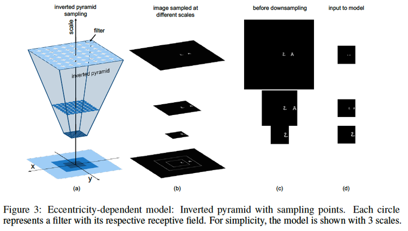
Scale pooling reduces the number of scales by taking the maximum value of corresponding locations in the feature maps across multiple scales. We set the spatial pooling constant using At end pooling, as described above. The type of scale pooling is indicated by writing the number of scales remaining in each layer, e.g. 11-1-1-1-1. The three configurations tested for scale pooling are (1) at the beginning, in which all the different scales are pooled together after the first layer, 11-1-1-1-1 (2) progressively, 11-7-5-3-1 and (3) at the end, 11-11-11-11-1, in which all 11 scales are pooled together at the last layer.
Contrast Normalization
Since we have multiple scales of input image, we perform normalization such that the sum of the pixel intensities in each scale is in the same range [0,1] followed by dividing them by a factor proportional to the crop area.
Experiments and its Set-Up
The models are trained with back-propagation to recognize a set of objects, called targets and flankers act as clutter with respect to these target objects. The target objects are the even MNIST numbers having translational variance (shifted at different locations of the image along the horizontal axis). Examples of the target and flanker configurations is shown below:
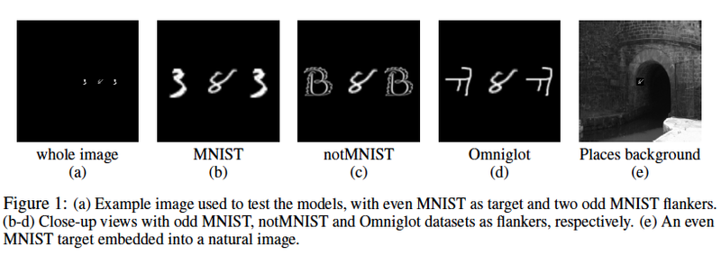
The target and the object are referred to as a and x respectively with the below four conifgurations: (1) No flankers. Only the target object. (a in the plots) (2) One central flanker closer to the center of the image than the target. (xa) (3) One peripheral flanker closer to the boundary of the image that the target. (ax) (4) Two flankers spaced equally around the target, being both the same object (xax).
DNNs trained with Target and Flankers
This is a constant spacing training setup where identical flankers are placed at a distance of 120 pixels either side of the target(xax) with the targte having translational variance. THe tests are evaluated on (i) DCNN with at the end pooling, and (ii) eccentricity-dependent model with 11-11-11-11-1 scale pooling, at the end spatial pooling and contrast normalization. The test data has different flanker configurations as described above.
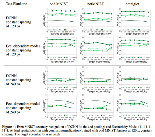
Observations
- With the flanker configuration same as the training one, models are better at recognizing objects in clutter rather than isolated objects for all image locations -If the target-flanker spacing is changed, then models perform worse -the eccentricity model is much better at recognizing objects in isolation than the DCNN because the multi-scale crops divide the image into discrete regions, letting the model learn from image parts as well as the whole image -Only the eccentricity-dependent model is robust to different flanker configurations not included in training, when the target is centered.
DNNs trained with Images with the Target in Isolation
Eccentric Model
Conclusions
We often think that just training the network with data similar to the test data would achieve good results in a general scenario too but thats not the case as we trained the model with flankers and it did not give us the ideal results for the target obects.
- Flanker Configuration: When models are trained with images of objects in isolation, adding flankers harms recognition. Adding two flankers is the same or worse than adding just one and the smaller the spacing between flanker and target, the more crowding occurs. These is because the pooling operation merges nearby responses, such as the target and flankers if they are close.
- Similarity between target and flanker: Flankers more similar to targets cause more crowding, because of the selectivity property of the learned DNN filters.
- Dependence on target location and contrast normalization: In DCNNs and eccentricitydependent models with contrast normalization, recognition accuracy is the same across all eccentricities. In eccentricity-dependent networks without contrast normalization, recognition does not decrease despite presence of clutter when the target is at the center of the image.
- Effect of pooling: adding pooling leads to better recognition accuracy of the models. Yet, in the eccentricity model, pooling across the scales too early in the hierarchy leads to lower accuracy.