summary

XGBoost: A Scalable Tree Boosting System

Presented by

Jiang, Cong

Song, Ziwei

Ye, Zhaoshan

Zhang, Wenling

Introduction

The Extreme Gradiant Boosting, also known as XGBoost, has been the leading model that dominates Kaggle, as well as other machine learning and data mining challenges. The main reason to its success is that this tree boosting system is highly scalable , which means it could be used to solve various problems with significantly less time and fewer resources.

This paper is written by the father of XGBoost, Tianqi Chen. It gives us an overview on how he used algorithmic optimizations as well as some important systems to develop XGBoost. He explained it in the following manner:

1. Based on gradient tree boosting algorithm, Chen makes some modifications to the regularized objective function and introduces an end-to-end tree boosting system. He also applies shrinkage and feature subsampling to prevent overfitting,

2. The system supports existing split finding algorithms including exact greedy and approximate algorithms. For weighted data, Chen proposes a distributed weighted quantile sketch algorithm which is provable; while for sparse data, he develops a novel sparsity-aware algorithm which is much faster than the naive model.

3. Storing the data in blocks is Chen's method to reduce sorting cost. The cache-aware block structure is highly effective for out-of-core tree learning.

4. XGBoost is evaluated by designed experiments with 4 datasets. Chen compares it with adjusted setting as well as other systems to test its performance.

Tree Boosting

Regularized Learning Objective

Suppose the given data set has m features and n examples. A tree ensemble model uses K additive functions to predict the output.

eq1.png

where F is the space of regression trees(CART). The author suggests the following regularized objective function to make improvements comparing to gradient boosting

eq2.png

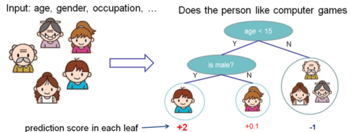
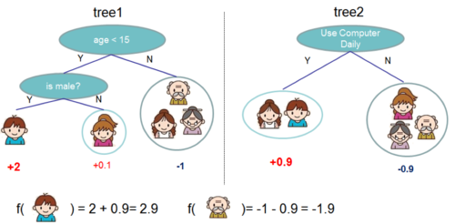
Regression tree contains continuous scores on each leaf, which is different with decision trees we have learned in class. The following 2 figures represent how to use the decision rules in the trees to classify it into the leaves and calculate the final prediction by summing up the score in the corresponding leaves.

Figure 0: Prediction Score of Tree Structure.

Figure 1: Tree Ensemble Model. The final prediction for a given example is the sum of predictions from each tree.

Gradient Tree Boosting

The tree ensemble model (Equation 2.) is trained in an additive manner. We need to add a new [math]\displaystyle{ f }[/math] to our objective.

eq2.2.png

After applying the second-order Taylor expansion to the above formula and removing constant terms, we can finally have

eq3.png

Define [math]\displaystyle{ I_{j} = \{i| q(X_{i}) \} }[/math] As the instance set of leaf j. We can rewrite Equation (3) as

eq4.png

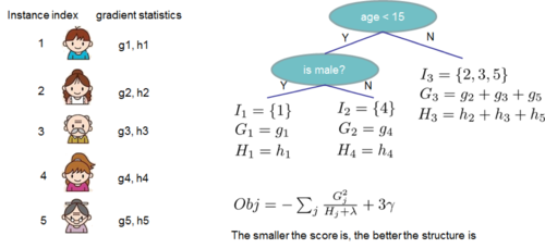
By computing the optimal weight and corresponding optimal value, we can use following equation as the scoring function which can measure the quality of a tree structure. Lower score means better tree structure.

eq5.png

The following figure shows an example how this score is calculated.

Figure 2: Structure Score Calculation. We only need to sum up the gradient and second order gradient statistics on each leaf, then apply the scoring formula to get the quality score.

Normally it is impossible to enumerate all the possible tree structures. Assume [math]\displaystyle{ I_{L} }[/math] and [math]\displaystyle{ I_{R} }[/math] are the instance sets of left and right nodes after the split, and [math]\displaystyle{ I = I_{L} + I_{R} }[/math]. Then the loss reduction after the split is given by

Shrinkage and Column Subsampling

In addition to the regularized objective, the paper also introduces two techniques to prevent over-fitting.

Method 1: Shrinkage. After each step of tree boosting, we scale newly added weights by a shrinkage factor η, which reduces the influence of every individual tree and leaves the space for future trees.

Method 2: Column (feature) subsampling. We try to build each individual tree with only a portion of predictors chosen randomly. This procedure encourages the variance between the trees (i.e. no same tree occurs). Implemented in an opensource packages, this method prevents over-fitting and speeds up the computations of parallel algorithm as well.

Split Finding Algorithms

The ways to find the best split can be realized by two main methods.

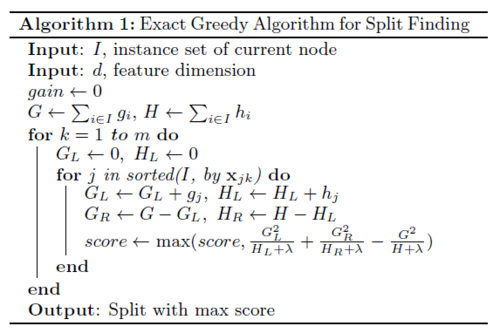
Basic exact greedy algorithm: enumerate over all the possible splits on all the features, which is computationally demanding. Sort the data first, and visit the data to accumulate the gradient statistics.

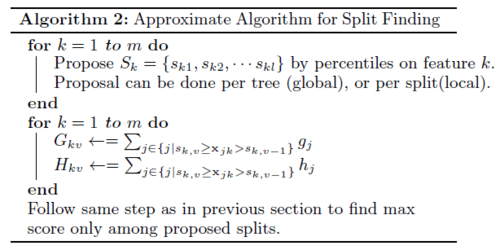
Approximate algorithm: To achieve an effective gradient tree boosting model, we first propose candidate splitting points by percentiles of feature distribution, map the continuous features into buckets split and then finds the best solution among the proposals by the aggregated statistics. The algorithm can be varied by the time the proposal is given. The global variant: all candidate splits are proposed at the initial phase of tree construction and used at all levels. The local variant: the candidate splits are refined after each splits. It is potential for deeper trees and it requires fewer candidates. Methods can be chosen according to users’ needs.

Evaluations

System Implementation

Implemented as an open source package, XGBoost is portable and reusable. Thus, it is available in various languages and ecosystems.

Dataset and Setup

Table 2 summarizes the 4 datasets used in the experiments.

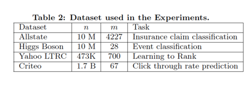
The first three datasets are used for the single machine parallel setting, which is run on a Dell PowerEdge R420 with two 8-core Intel Xeon and memory 64GB. Meanwhile, AWS c3.8xlarge machine is used for experiment in distributed and the out-of-core setting, which uses the criteo dataset. All available cores in the machines are devoted into the experiments, unless otherwise specified.

Multiple Experiments

The classification experiment uses Higgs Boson dataset to classify whether an event corresponds to the Higgs boson. The goal is to evaluate XGBoost using Exact Greedy Methods and compare it with column sampling XGBoost and two other well-known systems. Table 3 below summarizes the results.

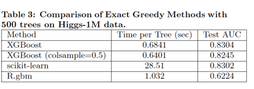
Overall, both XGBoost and scikit-learn performs better than R.gbm by 20% of Test AUC. In terms of time, however, XGBoost runs significantly faster than both scikit-learn and R.gbm. Note that XGBoost with column sampling performs slightly worse because the number of key features is limited. We could conclude that XGBoost using the exact greedy algorithm without column sampling works the best under this scenario.

The learning to rank experiment compares XGBoost(using exact greedy algorithm) with pGBRT(using approximate algorithm) in order to evaluate the system's performance on rank problem.

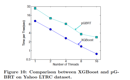
According to Table 4, XGBoost with column sampling performs almost as well as pGBRT, while using only 1/5 of the time. Note that pGBRT is the best previously published system to solve this rank problem.

The out-of-score and distributed experiments demonstrate XGBoost's ability to handle large data with a fast speed.

Source

**Sample format

Recurrent neural networks are a variation of deep neural networks that are capable of storing information about previous hidden states in special memory layers.<ref name=lstm> Hochreiter, Sepp, and Jürgen Schmidhuber. "Long short-term memory." Neural computation 9.8 (1997): 1735-1780. </ref> Unlike feed forward neural networks that take in a single fixed length vector input and output a fixed length vector output, recurrent neural networks can take in a sequence of fixed length vectors as input, because of their ability to store information and maintain a connection between inputs through this memory layer. By comparison, previous inputs would have no impact on current output for feed forward neural networks, whereas they can impact current input in a recurrent neural network. (This paper used the LSTM formulation from Graves<ref name=grave> Graves, Alex. "Generating sequences with recurrent neural networks." arXiv preprint arXiv:1308.0850 (2013). </ref>)

Where [math]\displaystyle{ \,S }[/math] is the base/source sentence, [math]\displaystyle{ \,T }[/math] is the paired translated sentence and [math]\displaystyle{ \,T_r }[/math] is the total training set. This objective function is to maximize the log probability of a correct translation [math]\displaystyle{ \,T }[/math] given the base/source sentence [math]\displaystyle{ \,S }[/math] over the entire training set. Once the training is complete, translations are produced by finding the most likely translation according to LSTM:

[math]\displaystyle{ \hat{T} = \underset{T}{\operatorname{arg\ max}}\ p(T|S) }[/math]

It has been showed that Long Short-Term Memory recurrent neural networks have the ability to generate both discrete and real-valued sequences with complex, long-range structure using next-step prediction <ref name=grave> Reference </ref>.