stat441w18/Convolutional Neural Networks for Sentence Classification: Difference between revisions
| Line 197: | Line 197: | ||
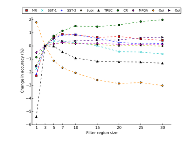
[[File:filter region size2.png|400px|thumb|center|Effect of several region sizes on MR dataset using non-static CNN | [[File:filter region size2.png|400px|thumb|center|Effect of several region sizes on MR dataset using non-static CNN | ||
(Zhang, Y. Wallace, B. 2016)]] | |||
Can using a different activation function aid performance? Several different activation functions are considered, but only best performing activations are reported below. The author only used ReLU. Here we can see that other activation functions can give us better results. | |||
[[File:activation.png|400px|thumb|center|Performance of different activation functions | |||
(Zhang, Y. Wallace, B. 2016)]] | |||
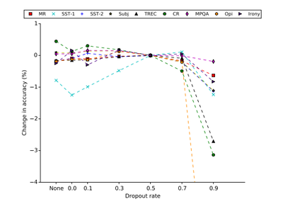
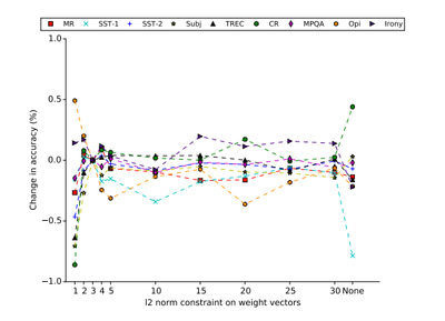
How effective is regularization? Tuning regularization seems to have little effect. | |||
[[File:droupout rate.png|400px|thumb|center|Effect of dropout rate | |||
(Zhang, Y. Wallace, B. 2016)]] | |||
[[File:l2 norm.png|400px|thumb|center|Effect of l2 norm constraint on weight vectors. | |||
(Zhang, Y. Wallace, B. 2016)]] | (Zhang, Y. Wallace, B. 2016)]] | ||
Revision as of 00:07, 13 March 2018
Presented by
1. Ben Schwarz
2. Cameron Miller
3. Hamza Mirza
4. Pavle Mihajlovic
5. Xiaowen Shi
6. Yitian Wu
7. Zekai Shao
Introduction
Deep learning is being used widely in visual and speech recognition and Natural Language Processing (NLP) has already became an important topic of research in this field. Most of the work performed for this revolves around learning word embeddings and completing compositions over the learned material.
The work for this paper obtained unsupervised word to vectors that were trained on the 100 billion publicly available words on google news. These words were then used to train a simple CNN with one layer of convolution. The simple model achieved excellent results and even with just little tuning of the hyper parameters. This suggests that pre-trained vectors can be effectively utilized for classification tasks.
The simple model was tested on various datasets such as movie reviews, Stanford Sentiment Treebank and customer reviews. Despite its limitations, the results were competitive to more complex models that use pooling schemes.
Model
Theory of Convolutional Neural Networks
Let [math]\displaystyle{ \boldsymbol{x}_{i:i+j} }[/math] represents the concatenation of words [math]\displaystyle{ \boldsymbol{x}_i, \boldsymbol{x}_{i+1}, \dots, \boldsymbol{x}_{i+j} }[/math] with concatenation operation [math]\displaystyle{ \oplus }[/math], [math]\displaystyle{ \boldsymbol{x}_{i:i+j} = \boldsymbol{x}_i \oplus \boldsymbol{x}_{i+1} \oplus \dots \oplus \boldsymbol{x}_{i+j} }[/math]. Then, a sentence of length [math]\displaystyle{ n }[/math] is a concatenation of [math]\displaystyle{ n }[/math] words, denoted as [math]\displaystyle{ \boldsymbol{x}_{1:n} }[/math], [math]\displaystyle{ \boldsymbol{x}_{1:n} = \boldsymbol{x}_1 \oplus \boldsymbol{x}_2 \oplus \dots \oplus \boldsymbol{x}_n }[/math]. Let [math]\displaystyle{ \boldsymbol{x}_i \in \mathbb{R}^k }[/math] denote the [math]\displaystyle{ i }[/math]-th word in the sentence, [math]\displaystyle{ i \in \{ 1, \dots, n \} }[/math].
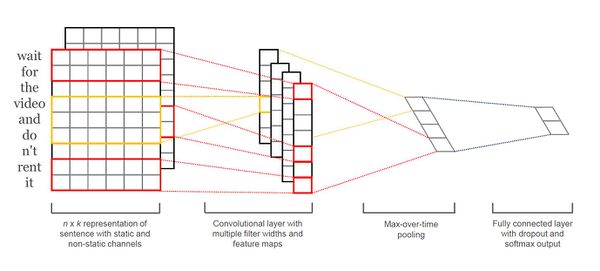
A Convolutional Neural Network (CNN) is a nonlinear function [math]\displaystyle{ f: \mathbb{R}^{hk} \to \mathbb{R} }[/math] that computes a series of outputs [math]\displaystyle{ c_i }[/math] from windows of [math]\displaystyle{ h }[/math] words [math]\displaystyle{ \boldsymbol{x}_{i:i+h-1} }[/math] in the sentence. [math]\displaystyle{ c_i = f \left( \boldsymbol{w} \cdot \boldsymbol{x}_{i:i+h-1} + b \right) }[/math], where [math]\displaystyle{ \boldsymbol{w} \in \mathbb{R}^{hk} }[/math] is call a filter and [math]\displaystyle{ b \in \mathbb{R} }[/math] is a bias term, [math]\displaystyle{ i \in \{ 1, \dots, n-h+1 \} }[/math]. The outputs form a [math]\displaystyle{ (n-h+1) }[/math]-dimensional vector [math]\displaystyle{ \boldsymbol{c} = \left[ c_1, c_2, \dots, c_{n-h+1} \right] }[/math], called a feature map.
To capture the most important feature from a feature map, we take the maximum value [math]\displaystyle{ \hat{c} = max \{ \boldsymbol{c} \} }[/math]. Since each filter corresponds to one feature, we obtain several features from multiple filters the model uses which form a penultimate layer. The penultimate layer then gets passed into a fully connected softmax layer which produces the probability distribution over labels.
Below is a slight variant of CNN with two "channels" of word vectors: static vectors and fine-tuned vectors via backpropagaton. We calculate [math]\displaystyle{ c_i }[/math] by applying each filter to both channels and then adding them together. The rest of the model is equivalent to a single channel CNN architecture as described above.
Model Regularization
To prevent co-adaptation and overfitting, we randomly drop out some hidden units on penultimate layer by setting them to zero during forward propagation and restrict the [math]\displaystyle{ l_2 }[/math]-norm of the weight vectors.
For example, consider a penultimate layer [math]\displaystyle{ \boldsymbol{l} }[/math] obtained from [math]\displaystyle{ m }[/math] filters, [math]\displaystyle{ \boldsymbol{l} = \left[ \hat{c}_1, \dots, \hat{c}_m \right] }[/math]. Let [math]\displaystyle{ \boldsymbol{u} \in \mathbb{R}^m }[/math] be a weight vector, [math]\displaystyle{ \boldsymbol{r} \in \mathbb{R}^m }[/math] be a "dropout" vector of Bernoulli random variables with a proportion of [math]\displaystyle{ p }[/math] being 1, and [math]\displaystyle{ \circ }[/math] be an element-wise multiplication operator. In forward propagation, instead of using [math]\displaystyle{ y = \boldsymbol{u} \cdot \boldsymbol{l} + b }[/math], we use [math]\displaystyle{ y = \boldsymbol{u} \cdot \left( \boldsymbol{l} \circ \boldsymbol{r} \right) + b }[/math] to obtain the output [math]\displaystyle{ y }[/math]. Gradients are only backpropagated through "remaining" units. Then at testing, we scale the learned weight vector by [math]\displaystyle{ p }[/math] such that [math]\displaystyle{ \hat{\boldsymbol{u}} = p\boldsymbol{u} }[/math]. We use [math]\displaystyle{ \hat{\boldsymbol{u}} }[/math] to score dropout sentences. Additionally, at each gradient descent step, we restrict [math]\displaystyle{ \| \boldsymbol{u} \|_2 = s }[/math] if [math]\displaystyle{ \| \boldsymbol{u} \|_2 \gt s }[/math].
Datasets and Experimental Setup

There are various benchmark for classification, for example:
MR:
Movie reviews with one sentence per review.
Class: positive/negative (Pang and Lee, 2005).
SST-1:
Standford Sentiment Treebank (An extension of MR) with train/dev*/test splits.
Classes: very positive, positive, neutral, negative, very negative.
dev set *: The set used for selecting the best performing model. (re-labeled by Socher er al. 2013)
SST-2:
Same as SST-1 but with neutral reviews removed and binary labels.
Class: positive/negative
Subj:
To classify a sentence as subjective or objective.
Class: subjective/objective (Pang and Lee, 2004)
TREC:
TREC question dataset, classifying a question into 6 question types
Class: question about person, location, numeric information. etc (Li and Roth, 2002).
CR:
Customer review towards various products (i.e. cameras, MP3 etc.).
Class: positive/negative reviews. (Hu and Liiu, 2004)
MPQA:
Opinion polarity detection subtask of the MPQA dataset.
(Wiebe et al., 2005).
Hyperparameters and Training
If no dev set is specified, then randomly pick 10 percent of training set as the dev set.
Using grid search, we find out the best combination of hyperparameters. On dev set of SST-2 dev set, we set all the hyperparameters: rectified linear units, filter windows(h) of 3, 4, 5 with 100 feature maps each, dropout rate (p) of 0.5, l2 constraint (s) of 3, and mini-batch size of 50.
Training is done through stochastic gradient descent over mini-batches with the Adadelta update rule(Zeiler, 2012)
Pre-trained Word Vectors
It is a popular method to initialize word vector through an unsupervised neural language model, which improves performance in the absence of a large supervised training set (Collobert et al ., 2011; Socher et al., 2011; lyyer et al,. 2014).
We use 'word2vec' vectors that were trained on 100 billion words from Google News. The vectors have dimensionality of 300 and were trained using bag-of-words architecture*( Mikolov et al., 2013). For words not present in the set of pre-trained words, we initialized them randomly.
Model Variations
CNN-rand:
baseline model where all words are randomly initialized and then modified during training
CNN-static:
model with pre-trained vectors from 'word2vec'(publicly available).
All words are randomly initialized and are kept static and the other parameters of the model are learned
CNN-non-static:
same as above but the pre-trained vectors are fine-tuned for each task
CNN-multichannel:
A model with two sets of word vectors.
Each set is a 'channel' and each filter is applied on both channels. One channel is fine-tuned via back-propagation, and the other is static(unchanged).
Both channels are initialized from 'word2vec'.
We keep other sources of randomness uniform within each datasets(such as CV-fold assignment, initialization of unknown word vectors, initialization of CNN parameters) to eliminate the effect of the above variations versus other random factors.
Training and Results
Scoring Method
The results of the CNN models against other methods can be seen in Table A. The accuracy of the four model variations of the CNN described above are compared with the accuracy (on a scale of 0 to 100) of various other methods.

Results
The baseline model (CNN-rand) with all randomly initialized words does not perform well compared to the other models as expected. In many cases, the baseline model performs the worst or close to the worst. Much to the surprise of the authors, the model with static vectors (CNN-static) performed exceptionally well, even against more sophisticated models from other research studies which have used static representations. As we will talk about, this suggests that pre-trained vectors are a useful ‘universal’ feature, that can be used against various datasets to improve accuracy.
The Effect of the Multichannel Model
One of the primary goals of the multichannel model was to prevent the issue of overfitting, and as a consequence, provide better results than the single channel. The idea was limit the deviation of learned vectors from the original values. The results of the experiments, however, did not show any significant evidence that the multichannel model performed better than the single channel models. In fact, there were some experiments in which single channel models scored better than the multichannel model, and some where the multichannel model scored better than the single channel models.
The Effects of Static vs. Non-Static Models
One of the key differences observed between the static and non-static models is that the fine-tuning of vectors in the non-static model allowed it to make meaningful associations, based on expressions of sentiment and uses of various punctuation. On the other hand, the static channel made stronger association based on syntax. Based on the results, the non-static model generally performed better than the static channel.
Further Observations
The multiple filter widths and feature maps of the CNN results in much greater performance than other models with similar architecture. Another feature of the CNN that improved performance was dropout, on average adding between 2-4% accuracy. When initializing words not in the word2vec vectors, performance was improved by sampling each dimension from [-a,a], where a is a value chosen to ensure the randomly initialized vectors and the ore-trained vectors have the same variance.
Criticisms
The author has acknowledged that at the time of his original experiments he did not have access to a GPU and thus could not run many differing experiments. Therefore the paper is missing things like ablation studies, which refers to removing/adding some feature of the model/algorithm and seeing how that can affect performance of the CNN (e.g. dropout rate). When a model is assessed it would be vital for the author to replicate the k-fold cross validation procedure and include ranges and variances of the performance. The author only reported the mean of the CV results but this overlooks the randomness of the stochastic processes which were used. This paper did not report variances despite using stochastic gradient descent, random dropout and random weight parameter initialization, which are all highly stochastic learning procedures. For more on an exhaustive analysis of model variants on CNNs Ye Zhang and Byron C. Wallace did a sensitivity analysis of CNNs for sentence classification (https://arxiv.org/pdf/1510.03820.pdf).
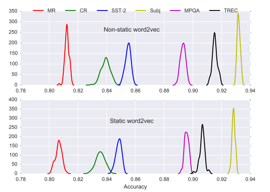
How does using different word vector representations effect the results? The only datasets of interest here are the first 7 from the table. Other word vector representations perform almost exactly the same. However not always true depending on the classification task. Here word2vec performs the best 4/9 times, glove performs the best 3/9 times and word2vec + glove performs best 2/9 (for the Subj set it performed only 0.02 better than the next best), this suggests that simply concatenating both representations together is not helpful.

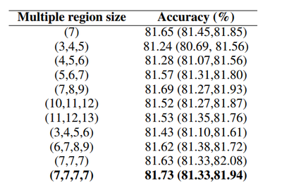
Does changing the filter region size have an effect on performance? Each set seems to have a distinct optimal filter region size. Parameterizing the region size and number of regions has a unique effect on each dataset. It seems to be a good idea to first find a single filter region size that lends the best accuracy and then looking for combinations of region sizes close to the single best size to optimize the performance.
Can using a different activation function aid performance? Several different activation functions are considered, but only best performing activations are reported below. The author only used ReLU. Here we can see that other activation functions can give us better results.

How effective is regularization? Tuning regularization seems to have little effect.
More Formulations/New Concepts
Learning to apply CNN on word embeddings, keeping track of the dimensions of the matrices can be confusing. The aim of this short post is to simply keep track of these dimensions and understand how CNN works for sentence classification. We would use a one-layer CNN on a 7-word sentence, with word embeddings of dimension 5 — a toy example to aid the understanding of CNN.
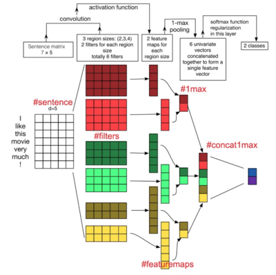
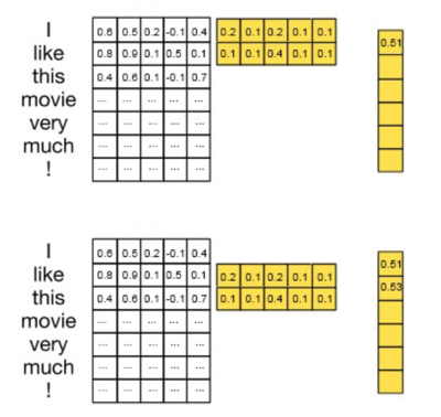
First, the two-word filter, represented by the 2 x 5 yellow matrix w, overlays across the word vectors of “I” and “like”. Next, it performs an element-wise product for all its 2 x 5 elements, and then sum them up and obtain one number (0.6 x 0.2 + 0.5 x 0.1 + … + 0.1 x 0.1 = 0.51). 0.51 is recorded as the first element of the output sequence, o, for this filter. Then, the filter moves down 1 word and overlays across the word vectors of ‘like’ and ‘this’ and perform the same operation to get 0.53. Therefore, o will have the shape of (s–h+1 x 1), in this case (7–2+1 x 1) To obtain the feature map, c, we add a bias term (a scalar, i.e., shape 1×1) and apply an activation function (e.g. ReLU). This gives us c, with the same shape as o (s–h+1 x 1).
Methods for Hyperparameter optimization:
Grid search
The traditional way of performing hyperparameter optimization has been grid search, or a parameter sweep, which is simply an exhaustive searching through a manually specified subset of the hyperparameter space of a learning algorithm. A grid search algorithm must be guided by some performance metric, typically measured by cross-validation on the training set or evaluation on a held-out validation set. Since the parameter space of a machine learner may include real-valued or unbounded value spaces for certain parameters, manually set bounds and discretization may be necessary before applying grid search. For example, a typical soft-margin SVM classifier equipped with an RBF kernel has at least two hyperparameters that need to be tuned for good performance on unseen data: a regularization constant C and a kernel hyperparameter γ. Both parameters are continuous, so to perform grid search, one selects a finite set of "reasonable" values for each, say C and γ. Grid search then trains an SVM with each pair (C, γ) in the Cartesian product of these two sets and evaluates their performance on a held-out validation set (or by internal cross-validation on the training set, in which case multiple SVMs are trained per pair). Finally, the grid search algorithm outputs the settings that achieved the highest score in the validation procedure. Grid search suffers from the curse of dimensionality, but is often embarrassingly parallel because typically the hyperparameter settings it evaluates are independent of each other
Random search
Since grid searching is an exhaustive and therefore potentially expensive method, several alternatives have been proposed. In particular, a randomized search that simply samples parameter settings a fixed number of times has been found to be more effective in high-dimensional spaces than exhaustive search. This is because oftentimes, it turns out some hyperparameters do not significantly affect the loss. Therefore, having randomly dispersed data gives more "textured" data than an exhaustive search over parameters that ultimately do not affect the loss.
Continuous bag- of-words architecture:
The input to the model could be wi−2,wi−1,wi+1,wi+2, the preceding and following words of the current word we are at. The output of the neural network will be wi. Hence you can think of the task as "predicting the word given its context"
Consider the training corpus having the following sentences: “the dog saw a cat”, “the dog chased the cat”, “the cat climbed a tree”
The corpus vocabulary has eight words. Once ordered alphabetically, each word can be referenced by its index. Let us assume that we decide to use three neurons in the hidden layer. This means that WI and WO will be 8×3 and 3×8 matrices, respectively. Suppose we want the network to learn relationship between the words “cat” and “climbed”. That is, the network should show a high probability for “climbed” when “cat” is inputted to the network. In word embedding terminology, the word “cat” is referred as the context word and the word “climbed” is referred as the target word. In this case, the input vector X will be [0 1 0 0 0 0 0 0]^t. Notice that only the second component of the vector is 1. This is because the input word is “cat” which is holding number two position in sorted list of corpus words. Given that the target word is “climbed”, the target vector will look like [0 0 0 1 0 0 0 0 ]^t.
Let X^tWIWO = [0.143073 0.094925 0.114441 0.111166 0.149289 0.122874 0.119431 0.144800]
is a 1×8 matrix which represents the probabilities for eight words in the corpus. In essence, this is how Word2vec learns relationships between words and in the process develops vector representations for words in the corpus.
Conclusion
Yoon Kim described a series of experiments with CNNs using word2vec for differing types of sentence classifications. With minimal hyperparameter tuning and a simple CNN with 1 layer of convolution the models performed in some cases better than the other established benchmarks. The author was able to beat the provided benchmarks in 4/7 datasets effectively demonstrating the power of CNNs for sentence classification.
Source
Kim, Y. (2014). Convolutional Neural Networks for Sentence Classification. Retrieved from https://arxiv.org/pdf/1408.5882.pdf. arXiv:1408.5882v2 [cs.CL].
Zhang, Y. Wallace, B. (2016). A Sensitivity Analysis of (and Practitioners' Guide to) Convolutional Neural Networks for Sentence Classification. Retrieved from https://arxiv.org/pdf/1510.03820.pdf. arVix:1510.03820v4 [cs.CL].