Wasserstein Auto-Encoders

Introduction

Recent years have seen a convergence of two previously distinct approaches: representation learning from high dimensional data, and unsupervised generative modeling. In the field that formed at their intersection, Variational Auto-Encoders (VAEs) and Generative Adversarial Networks (GANs) have emerged to become well-established. VAEs are theoretically elegant but with the drawback that they tend to generate blurry samples when applied to natural images. GANs on the other hand produce better visual quality of sampled images, but come without an encoder, are harder to train and suffer from the mode-collapse problem when the trained model is unable to capture all the variability in the true data distribution. Thus there has been a push to come up with the best way to combine them together, but a principled unifying framework is yet to be discovered.

This work proposes a new family of regularized auto-encoders called the Wasserstein Auto-Encoder (WAE). The proposed method provides a novel theoretical insight into setting up an objective function for auto-encoders from the point of view of of optimal transport (OT). This theoretical formulation leads the authors to examine adversarial and maximum mean discrepancy based regularizers for matching a prior and the distribution of encoded data points in the latent space. An empirical evaluation is performed on MNIST and CelebA datasets, where WAE is found to generate samples of better quality than VAE while preserving training stability, encoder-decoder structure and nice latent manifold structure.

The main contribution of the proposed algorithm is to provide theoretical foundations for using optimal transport cost as the auto-encoder objective function, while blending auto-encoders and GANs in a principled way. It also theoretically and experimentally explores the interesting relationships between WAEs, VAEs and adversarial auto-encoders.

Proposed Approach

Theory of Optimal Transport and Wasserstein Distance

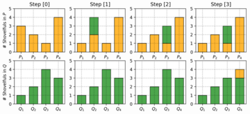
Wasserstein Distance is a measure of the distance between two probability distributions. It is also called Earth Mover’s distance, short for EM distance, because informally it can be interpreted as moving piles of dirt that follow one probability distribution at a minimum cost to follow the other distribution. The cost is quantified by the amount of dirt moved times the moving distance. A simple case where the probability domain is discrete is presented below.

Step-by-step plan of moving dirt between piles in P and Q to make them match (W = 5).

When dealing with the continuous probability domain, the EM distance or the minimum one among the costs of all dirt moving solutions becomes: \begin{align} \small W(p_r, p_g) = \underset{\gamma\sim\Pi(p_r, p_g)} {\inf}\pmb{\mathbb{E}}_{(x,y)\sim\gamma}[\parallel x-y\parallel] \end{align} The Wasserstein distance or the cost of Optimal Transport (OT) provides a much weaker topology, which informally means that it makes it easier for a sequence of distribution to converge as compared to other f-divergences. This is particularly important in applications where data is supported on low dimensional manifolds in the input space. As a result, stronger notions of distances such as KL-divergence, often max out, providing no useful gradients for training. In contrast, OT has a much nicer linear behavior even upon saturation.

Problem Formulation and Notation

In this paper, calligraphic letters, i.e. [math]\displaystyle{ \small {\mathcal{X}} }[/math], are used for sets, capital letters, i.e. [math]\displaystyle{ \small X }[/math], are used for random variables and lower case letters, i.e. [math]\displaystyle{ \small x }[/math], for their values. Probability distributions are denoted with capital letters, i.e. [math]\displaystyle{ \small P(X) }[/math], and corresponding densities with lower case letters, i.e. [math]\displaystyle{ \small p(x) }[/math].

This work aims to minimize OT [math]\displaystyle{ \small W_c(P_X, P_G) }[/math] between the true (but unknown) data distribution [math]\displaystyle{ \small P_X }[/math] and a latent variable model [math]\displaystyle{ \small P_G }[/math] specified by the prior distribution [math]\displaystyle{ \small P_Z }[/math] of latent codes [math]\displaystyle{ \small Z \in \pmb{\mathbb{Z}} }[/math] and the generative model [math]\displaystyle{ \small P_G(X|Z) }[/math] of the data points [math]\displaystyle{ \small X \in \pmb{\mathbb{X}} }[/math] given [math]\displaystyle{ \small Z }[/math].

Kantorovich's formulation of the OT problem is given by: \begin{align} \small W_c(P_X, P_G) := \underset{\Gamma\sim {\mathcal{P}}(X \sim P_X, Y \sim P_G)}{\inf} {\pmb{\mathbb{E}}_{(X,Y)\sim\Gamma}[c(X,Y)]} \end{align} where [math]\displaystyle{ \small c(x,y) }[/math] is any measurable cost function and [math]\displaystyle{ \small {\mathcal{P}(X \sim P_X,Y \sim P_G)} }[/math] is a set of all joint distributions of [math]\displaystyle{ \small (X,Y) }[/math] with marginals [math]\displaystyle{ \small P_X }[/math] and [math]\displaystyle{ \small P_G }[/math]. When [math]\displaystyle{ \small c(x,y)=d(x,y) }[/math], the following Kantorovich-Rubinstein duality holds for the [math]\displaystyle{ \small 1^{st} }[/math] root of [math]\displaystyle{ \small W_c }[/math]: \begin{align} \small W_1(P_X, P_G) := \underset{f \in {\mathcal{F_L}}} {\sup} {\pmb{\mathbb{E}}_{X \sim P_X}[f(X)]} -{\pmb{\mathbb{E}}_{Y \sim P_G}[f(Y)]} \end{align} where [math]\displaystyle{ \small {\mathcal{F_L}} }[/math] is the class of all bounded Lipschitz continuous functions.

Wasserstein Auto-Encoders

The proposed method focuses on latent variables [math]\displaystyle{ \small P_G }[/math] defined by a two step procedure, where first a code [math]\displaystyle{ \small Z }[/math] is sampled from a fixed prior distribution [math]\displaystyle{ \small P_Z }[/math] on a latent space [math]\displaystyle{ \small {\mathcal{Z}} }[/math] and then [math]\displaystyle{ \small Z }[/math] is mapped to the image [math]\displaystyle{ \small X \in {\mathcal{X}} }[/math] with a transformation. This results in a density of the form \begin{align} \small p_G(x) := \int_{{\mathcal{Z}}} p_G(x|z)p_z(z)dz, \forall x\in{\mathcal{X}} \end{align} assuming all the densities are properly defined. It turns out that if the focus is only on generative models deterministically mapping [math]\displaystyle{ \small Z }[/math] to [math]\displaystyle{ \small X = G(Z) }[/math], then the OT cost takes a much simpler form as stated below by Theorem 1.

Theorem 1 For any function [math]\displaystyle{ \small G:{\mathcal{Z}} \rightarrow {\mathcal{X}} }[/math], where [math]\displaystyle{ \small Q(Z) }[/math] is the marginal distribution of [math]\displaystyle{ \small Z }[/math] when [math]\displaystyle{ \small X \in P_X }[/math] and [math]\displaystyle{ \small Z \in Q(Z|X) }[/math], \begin{align} \small \underset{\Gamma\sim {\mathcal{P}}(X \sim P_X, Y \sim P_G)}{\inf} {\pmb{\mathbb{E}}_{(X,Y)\sim\Gamma}[c(X,Y)]} = \underset{Q : Q_z=P_z}{\inf} {{\pmb{\mathbb{E}}_{P_X}}{\pmb{\mathbb{E}}_{Q(Z|X)}}[c(X,G(Z))]} \end{align} This essentially means that instead of finding a coupling [math]\displaystyle{ \small \Gamma }[/math] between two random variables living in the [math]\displaystyle{ \small {\mathcal{X}} }[/math] space, one distributed according to [math]\displaystyle{ \small P_X }[/math] and the other one according to [math]\displaystyle{ \small P_G }[/math], it is sufficient to find a conditional distribution [math]\displaystyle{ \small Q(Z|X) }[/math] such that its [math]\displaystyle{ \small Z }[/math] marginal [math]\displaystyle{ \small Q_Z(Z) := {\pmb{\mathbb{E}}_{X \sim P_X}[Q(Z|X)]} }[/math] is identical to the prior distribution [math]\displaystyle{ \small P_Z }[/math]. In order to implement a numerical solution to Theorem 1, the constraints on [math]\displaystyle{ \small Q(Z|X) }[/math] and [math]\displaystyle{ \small P_Z }[/math] are eased and a penalty function is added to the objective leading to the WAE objective function given by:

\begin{align} \small D_{WAE}(P_X, P_G):= \underset{Q(Z|X) \in Q}{\inf} {{\pmb{\mathbb{E}}_{P_X}}{\pmb{\mathbb{E}}_{Q(Z|X)}}[c(X,G(Z))]} + {\lambda} {\cdot} {{\mathcal{D}}_Z(Q_Z,P_Z)} \end{align} where [math]\displaystyle{ \small Q }[/math] is any non-parametric set of probabilistic encoders, [math]\displaystyle{ \small {\mathcal{D}}_Z }[/math] is an arbitrary divergence between [math]\displaystyle{ \small Q_Z }[/math] and [math]\displaystyle{ \small P_Z }[/math], and [math]\displaystyle{ \small \lambda \gt 0 }[/math] is a hyperparameter. The authors propose two different penalties [math]\displaystyle{ \small {\mathcal{D}}_Z(Q_Z,P_Z) }[/math] based on adversarial training (GANs) and maximum mean discrepancy (MMD).

WAE-GAN: GAN-based

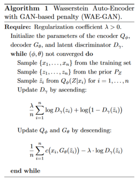
The first option is to choose [math]\displaystyle{ \small {\mathcal{D}}_Z(Q_Z,P_Z) = D_{JS}(Q_Z,P_Z) }[/math], where [math]\displaystyle{ \small D_{JS} }[/math] is the Jensen-Shannon divergence metric, and use adversarial training to estimate it. Specifically a discriminator is introduced in the latent space [math]\displaystyle{ \small {\mathcal{Z}} }[/math] trying to separate true points sampled from [math]\displaystyle{ \small P_Z }[/math] from fake ones sampled from [math]\displaystyle{ \small Q_Z }[/math]. This results in Algorithm 1. It is interesting that the min-max problem is moved from the input pixel space to the latent space.

WAE-MMD: MMD-based

For a positive definite kernel [math]\displaystyle{ \small k: {\mathcal{Z}} \times {\mathcal{Z}} \rightarrow {\mathcal{R}} }[/math], the following expression is called the maximum mean discrepancy: \begin{align} \small MMD_k(P_Z,Q_Z) = \parallel \int_{{\mathcal{Z}}} k(z,\cdot)dP_z(z) - \int_{{\mathcal{Z}}} k(z,\cdot)dQ_z(z) \parallel \end{align} This can be used as a divergence measure and the authors propose to use [math]\displaystyle{ \small {\mathcal{D}}_Z(Q_Z,P_Z) = MMD_k(P_Z,Q_Z) }[/math], which leads to Algorithm 2.