A Neural Representation of Sketch Drawings

Introduction

There have been many recent advances in neural generative models for low resolution pixel-based images. Humans, however, do not see the world in a grid of pixels and more typically communicate drawings of the things we see using a series of pen strokes that represent components of objects. These pen strokes are similar to the way vector-based images store data. This paper proposes a new method for creating conditional and unconditional generative models for creating these kinds of vector sketch drawings based on recurrent neural networks (RNNs). The paper explores many applications of these kinds of models, especially creative applications and makes available their unique dataset of vector images.

Related Work

Previous work related to sketch drawing generation includes methods that focussed primarily on converting input photographs into equivalent vector line drawings. Image generating models using neural networks also exist but focussed more on generation of pixel-based imagery. Some recent work has focussed on handwritten character generation using RNNs and Mixture Density Networks to generate continuous data points. This work has been extended somewhat recently to conditionally and unconditionally generate handwritten vectorized Chinese Kanji characters by modeling them as a series of pen strokes. Furthermore, this paper builds on work that employed Sequence-to-Sequence models with Variational Autencoders to model English sentences in latent vector space.

One of the limiting factors for creating models that operate on vector datasets has been the dearth of publicly available data. Previously available datasets include Sketch, a set of 20K vector drawings; Sketchy, a set of 70K vector drawings; and ShadowDraw, a set of 30K raster images with extracted vector drawings.

Methodology

Dataset

The “QuickDraw” dataset used in this research was assembled from 75K user drawings extracted from the game “Quick, Draw!” where users drew objects from one of hundreds of classes in 20 seconds or less. The dataset is split into 70K training samples and 2.5K validation and test samples each and represents each sketch a set of “pen stroke actions”. Each action is provided as a vector in the form [math]\displaystyle{ (\Delta x, \Delta y, p_{1}, p_{2}, p_{3}) }[/math]. For each vector, [math]\displaystyle{ \Delta x }[/math] and [math]\displaystyle{ \Delta y }[/math] give the movement of the pen from the previous point, with the initial location being the origin. The last three vector elements are a one-hot representation of pen states; [math]\displaystyle{ p_{1} }[/math] indicates that the pen is down and a line should be drawn between the current point and the next point, [math]\displaystyle{ p_{2} }[/math] indicates that the pen is up and no line should be drawn between the current point and the next point, and [math]\displaystyle{ p_{3} }[/math] indicates that the drawing is finished and subsequent points and the current point should not be drawn.

Sketch-RNN

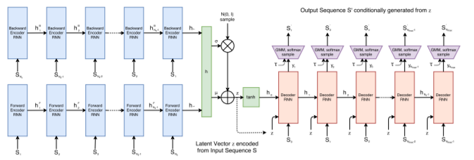
The model is a Sequence-to-Sequence Variational Autoencoder (VAE). The encoder model is a symmetric and parallel set of two RNNs that individually process the sketch drawings in forward and reverse order, respectively. The hidden state produced by each encoder model is then concatenated into a single hidden state [math]\displaystyle{ h }[/math].

The concatenated hidden state [math]\displaystyle{ h }[/math] is then projected into two vectors [math]\displaystyle{ \mu }[/math] and [math]\displaystyle{ \hat{\sigma} }[/math] each of size [math]\displaystyle{ N_{z} }[/math] using a fully connected layer. [math]\displaystyle{ \hat{\sigma} }[/math] is then converted into a non-negative standard deviation parameter [math]\displaystyle{ \sigma }[/math] using an exponential operator. These two parameters [math]\displaystyle{ \mu }[/math] and [math]\displaystyle{ \sigma }[/math] are then used along with an IID Gaussian vector distributed as [math]\displaystyle{ \mathcal{N}(0, I) }[/math] of size [math]\displaystyle{ N_{z} }[/math] to construct a random vector [math]\displaystyle{ z \in ℝ^{N_{z}} }[/math], similar to the method used for VAE: \begin{align} \mu = W_{\mu}h + b_{mu}\textrm{, }\hat{\sigma} = W_{\sigma}h + b_{\sigma}\textrm{, }\sigma = exp\bigg{(}\frac{\hat{\sigma}}{2}\bigg{)}\textrm{, }z = \mu + \sigma \odot \mathcal{N}(0,I) \end{align}

The decoder model is another RNN that samples output sketches from the latent vector [math]\displaystyle{ z }[/math]. The initial hidden states of each recurrent neuron are determined using [math]\displaystyle{ [h_{0}, c_{0}] = tanh(W_{z}z + b_{z}) }[/math]. Each step of the decoder RNN accepts the previous point [math]\displaystyle{ S_{i-1} }[/math] and the latent vector [math]\displaystyle{ z }[/math] as concatenated input. The initial point given is the origin point with pen state down. The output at each step are the parameters for a probability distribution of the next point [math]\displaystyle{ S_{i} }[/math]. Outputs [math]\displaystyle{ \Delta x }[/math] and [math]\displaystyle{ \Delta y }[/math] are modelled using a Gaussian Mixture Model (GMM) with M normal distributions and output pen states [math]\displaystyle{ (q_{1}, q_{2}, q_{3}) }[/math] modelled as a categorical distribution with one-hot encoding. \begin{align} P(\Delta x, \Delta y) = \sum_{j=1}^{M}\Pi_{j}\mathcal{N}(\Delta x, \Delta y | \mu_{x, j}, \mu_{y, j}, \sigma_{x, j}, \sigma_{y, j}, \rho_{xy, j})\textrm{, where }\sum_{j=1}^{M}\Pi_{j} = 1 \end{align}

For each of the M distributions in the GMM, parameters [math]\displaystyle{ \mu }[/math] and [math]\displaystyle{ \sigma }[/math] are output for both the x and y locations signifying the mean location of the next point and the standard deviation, respectively. Also output from each model is parameter [math]\displaystyle{ \rho_{xy} }[/math] signifying correlation of each bivariate normal distribution. An additional vector [math]\displaystyle{ \Pi }[/math] is an output giving the mixture weights for the GMM. The output [math]\displaystyle{ S_{i} }[/math] is determined from each of the mixture models using softmax sampling from these distributions.

One of the key difficulties in training this model is the highly imbalanced class distribution of pen states. In particular, the state that signifies a drawing is complete will only appear one time per each sketch and is difficult to incorporate into the model. In order to have the model stop drawing, the authors introduce a hyperparameter that limits the number of points per drawing to being no more than [math]\displaystyle{ N_{max} }[/math], after which all output states form the model are set to (0, 0, 0, 0, 1) to force the drawing to stop.

To sample from the model, the parameters required by the GMM and categorical distributions are generated at each time step and the model is sampled until a “stop drawing” state appears or the time state reaches time [math]\displaystyle{ N_{max} }[/math]. The authors also introduce a “temperature” parameter [math]\displaystyle{ \tau }[/math] that controls the randomness of the drawings by modifying the pen states, model standard deviations, and mixture weights as follows:

\begin{align} \hat{q}_{k} \rightarrow \frac{\hat{q}_{k}}{\tau}\textrm{, }\hat{\Pi}_{k} \rightarrow \frac{\hat{\Pi}_{k}}{\tau}\textrm{, }\sigma^{2}_{x} \rightarrow \sigma^{2}_{x}\tau\textrm{, }\sigma^{2}_{y} \rightarrow \sigma^{2}_{y}\tau \end{align}

This parameter [math]\displaystyle{ \tau }[/math] lies in the range (0, 1]. As the parameter approaches 0, the model becomes more deterministic and always produces the point locations with the maximum likelihood for a given timestep.

Unconditional Generation

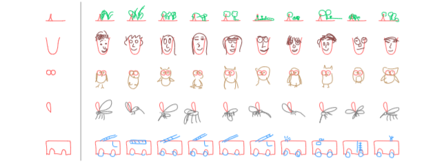
The authors also explored unconditional generation of sketch drawings by only training the decoder RNN module. To do this, the initial hidden states of the RNN were set to 0, and only vectors from the drawing input are used as input without any conditional latent variable [math]\displaystyle{ z }[/math]. Different sketches are sampled from the network by only varying the temperature parameter [math]\displaystyle{ \tau }[/math] between 0.2 and 0.9

Training

The training procedure follows the same approach as training for VAE and uses a loss function that consists of the sum of Reconstruction Loss [math]\displaystyle{ L_{R} }[/math] and KL Divergence Loss [math]\displaystyle{ L_{KL} }[/math]. The reconstruction loss term is composed of two terms; [math]\displaystyle{ L_{s} }[/math], which tries to maximize the log-likelihood of the generated probability distribution explaining the training data [math]\displaystyle{ S }[/math] and [math]\displaystyle{ L_{p} }[/math] which is the log loss of the pen state terms. \begin{align} L_{s} = -\frac{1}{N_{max}}\sum_{i=1}^{N_{S}}log\bigg{(}\sum_{j=1}^{M}\Pi_{j,i}\mathcal{N}(\Delta x_{i},\Delta y_{i} | \mu_{x,j,i},\mu_{y,j,i},\sigma_{x,j,i},\sigma_{y,j,i},\rho_{xy,j,i})\bigg{)} \end{align} \begin{align} L_{p} = -\frac{1}{N_{max}}\sum_{i=1}^{N_{max}} \sum_{k=1}^{3}p_{k,i}log(q_{k,i}) \end{align} \begin{align} L_{R} = L_{s} + L{p} \end{align}

The KL divergence loss [math]\displaystyle{ L_{KL} }[/math] measures the difference between the latent vector [math]\displaystyle{ z }[/math] and an IID Gaussian distribution with 0 mean and unit variance. This term, normalized by the number of dimensions [math]\displaystyle{ N_{z} }[/math] is calculated as: \begin{align} L_{KL} = -\frac{1}{2N_{z}}\big{(}1 + \hat{\sigma} - \mu^{2} – exp(\hat{\sigma})\big{)} \end{align}

The loss for the entire model is thus the weighted sum: \begin{align} Loss = L_{R} + w_{KL}L_{KL} \end{align}

The value of the weight parameter [math]\displaystyle{ w_{KL} }[/math] has the effect that as [math]\displaystyle{ w_{KL} \rightarrow 0 }[/math], there is a loss in ability to enforce a prior over the latent space and the model assumes the form of a pure autoencoder. As with VAEs, there is a trade-off between optimizing for the two loss terms (i.e. between how precisely the model can regenerate training data [math]\displaystyle{ S }[/math] and how closely the latent vector [math]\displaystyle{ z }[/math] follows a standard normal distribution) - smaller values of [math]\displaystyle{ w_{KL} }[/math] lead to better [math]\displaystyle{ L_R }[/math] and worse [math]\displaystyle{ L_{KL} }[/math] compared to bigger values of [math]\displaystyle{ w_{KL} }[/math].

Experiments

The authors trained multiple conditional and unconditional models using varying values of [math]\displaystyle{ w_{KL} }[/math] and recorded the different [math]\displaystyle{ L_{R} }[/math] and [math]\displaystyle{ L_{KL} }[/math] values at convergence. The network used LSTM as it’s encoder RNN and HyperLSTM as the decoder network. The HyperLSTM model was used for decoding because it has a history of being useful in sequence generation tasks. (A HyperLSTM consists of two coupled LSTMS: an auxiliary LSTM and a main LSTM. At every time step, the auxiliary LSTM reads the previous hidden state and the current input vector, and computes an intermediate vector [math]\displaystyle{ z }[/math]. The weights of the main LSTM used in the current time step are then a learned function of this intermediate vector [math]\displaystyle{ z }[/math]. That is, the weights of the main LSTM are allowed to vary between time steps as a function of the output of the auxiliary LSTM. See Ha et al. (2016) for details)

Conditional Reconstruction

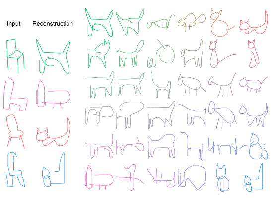
The authors qualitatively assessed the reconstructed images [math]\displaystyle{ S’ }[/math] given input sketch [math]\displaystyle{ S }[/math] using different values for the temperature hyperparameter [math]\displaystyle{ \tau }[/math]. The figure above shows the results for different values of [math]\displaystyle{ \tau }[/math] starting with 0.01 at the far left and increasing to 1.0 on the far right. Interestingly, sketches with extra features like a cat with 3 eyes are reproduced as a sketch of a cat with two eyes and sketches of object of a different class such as a toothbrush are reproduced as a sketch of a cat that maintains several of the input toothbrush sketches features.

Latent Space Interpolation

The latent space vectors [math]\displaystyle{ z }[/math] have few “gaps” between encoded latent space vectors due to the enforcement of a Guassian prior. This allowed the authors to do simple arithmetic on the latent vectors from different sketches and produce logical resulting images in the same style as latent space arithmetic on Word2Vec vectors.

Sketch Drawing Analogies

Given the latent space arithmetic possible, it was found that features of a sketch could be added after some sketch input was encoded. For example, a drawing of a cat with a body could be produced by providing the network with a drawing of a cat’s head, and then adding a latent vector to the embedding layer that represents “body”. As an example, this “body” vector might be produced by taking a drawing of a pig with a body and subtracting a vector representing the pigs head.

Predicting Different Endings of Incomplete Sketches

Using the decoder RNN only, it is possible to finish sketches by conditioning future vector line predictions on the previous points. To do this, the decoder RNN is first used to encode some existing points into the hidden state of the decoder network and then generating the remaining points of the sketch.

Applications and Future Work

Sketch-rnn may enable the production of several creative applications. These might include applications that help suggest ways an artist could finish a sketch, enable artists to explore latent space arithmetic to find interesting outputs given different sketch inputs, or allow the production of multiple different sketches of some object as a purely generative application. The authors suggest that providing some conditional sketch of an object to a model designed to produce output of a different class might be useful for producing sketches that morph the two different object classes into one sketch. For example, the image below was trained on drawing cats, but a chair was used as the input. This results in a chair looking cat.

Sketch-rnn may also be useful as a teaching tool to help people learn how to draw, especially if it were to be trained on higher quality images. Teaching tools might suggest to students how to proceed to finish a sketch, or intake low fidelity sketches to produce a higher quality and “more coherent” output sketch.

The authors noted that sketch-rnn is not as effective at generating coherent sketches when trained on a large number of classes simultaneously (experiments shown mostly used datasets consisting of one or two object classes), and plan to use class information outside the latent space to try to model a greater number of classes.

Finally the authors suggest that combining this model with another that produces photorealistic pixel-based images using sketch input, such as Pix2Pix may be an interesting direction for future research. In this case, the output from the sketch-rnn model would be used as input for Pix2Pix and could produce photorealistic images given some crude sketch from a user.

Conclusion

The authors presented sketch-rnn, a RNN model for modelling and generating vector-based sketch drawings. The VAE inspired architecture allows sampling the latent space to generate new drawings and also allows for applications that use latent space arithmetic in the style of Word2Vec to produce new drawings given operations on embedded sketch vectors. The authors also made available a large dataset of sketch drawings in the hope of encouraging more research in the area of vector-based image modelling.

Criticisms

The paper produces an interesting model that can effectively model vector-based images instead of traditional pixel-based images. This is an interesting problem because vector based images require producing a new way to encode the data. While the results from this paper are interesting, most of the techniques used are borrowed ideas from Variational Autoencoders and the main architecture is not terribly groundbreaking.

One novel part about the architecture presented was the way the authors used GMMs in the decoder network. While this was interesting and seemed to allow the authors to produce different outputs given the same latent vector input [math]\displaystyle{ z }[/math] by manipulating the [math]\displaystyle{ \tau }[/math] hyperparameter, it was not that clear in the article why GMMs were used instead of a more simple architecture. Much time was spent explaining basics about GMM parameters like [math]\displaystyle{ \mu }[/math] and [math]\displaystyle{ \sigma }[/math], but there was comparatively little explanation about how points were actually sampled from these mixture models.

Finally, the authors gloss somewhat over how they were able to encode previous sketch points using only the decoder network into the hidden state of the decoder RNN to finish partially finished sketches. I can only assume that some kind of back-propagation was used to encode the expected sketch points into the hidden parameters of the decoder, but no explanation was given in the paper.

Source

Ha, D., & Eck, D. A neural representation of sketch drawings. In Proc. International Conference on Learning Representations (2018).

Ha, David, Andrew Dai, and Quoc V. Le. "Hypernetworks." arXiv preprint arXiv:1609.09106 (2016).