stat946w18/AmbientGAN: Generative Models from Lossy Measurements

Introduction

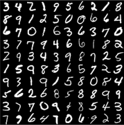
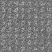
Generative Adversarial Networks operate by simulating complex distributions but training them requires access to large amounts of high quality data. Often times we only have access to noisy or partial observations, from here on referred to as measurements of the true data. If know the measurement function and we would like to train a generative model for the true data there are several ways to continue with varying degrees of success. We will use noisy MNIST data as an illustrative example. Suppose we only see MNIST data that have been run through a Gaussian kernel (blurred) with some noise from a [math]\displaystyle{ N(0, 0.5^2) }[/math] distribution added to each pixel:

• 

  True Data (Unobserved)

• 

  Measured Data (Observed)

Ignore the problem

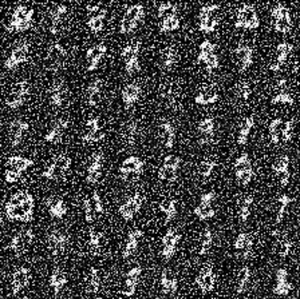
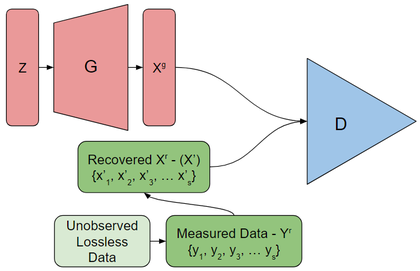
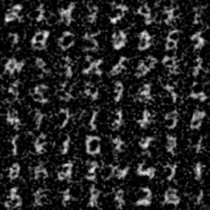
Train a generative model directly on the measured data. This will obviously be unable to generate the true distribution before measurement has occurred.

Try to recover the information lost

Works better than ignoring the problem but depends on how easily the measurement function can be inversed.

AmbientGAN

Ashish Bora, Eric Price and Alexandros G. Dimakis propose AmbientGAN as a way to recover the true underlying distribution from measurements of the true data.

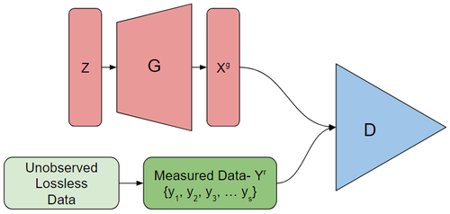
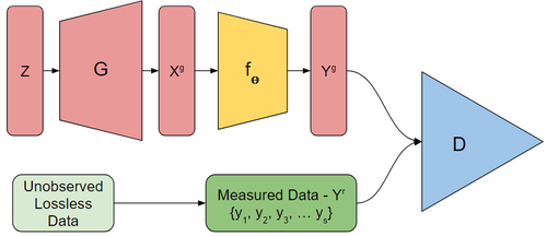
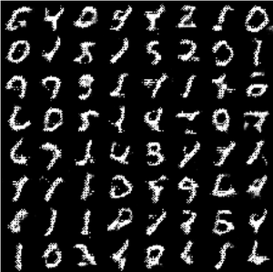
AmbientGAN works by training a generator which attempts to have the measruements of the output it generates fool the discriminator. The discriminator must distinguish between real and generated measurements.

Model

For the following variables superscript [math]\displaystyle{ r }[/math] represents the true distributions while superscript [math]\displaystyle{ g }[/math] represents the generated distributions. Let [math]\displaystyle{ x }[/math], represent the underlying space and [math]\displaystyle{ y }[/math] for the measurement.

Thus [math]\displaystyle{ p_x^r }[/math] is the real underlying distribution over [math]\displaystyle{ \mathbb{R}^n }[/math] that we are interested in. However if we assume our (known) measurement functions, [math]\displaystyle{ f_\theta: \mathbb{R}^n \to \mathbb{R}^m }[/math] are parameterized by [math]\displaystyle{ \theta \sim p_\theta }[/math], we can only observe [math]\displaystyle{ y = f_\theta(x) }[/math].

Mirroring the standard GAN setup we let [math]\displaystyle{ Z \in \mathbb{R}^k, Z \sim p_z }[/math] and [math]\displaystyle{ \Theta \sim p_\theta }[/math] be random variables coming from a distribution that is easy to sample.

If we have a generator [math]\displaystyle{ G: \mathbb{R}^k \to \mathbb{R}^n }[/math] then we can generate [math]\displaystyle{ X^g = G(Z) }[/math] which has distribution [math]\displaystyle{ p_x^g }[/math] a measurement [math]\displaystyle{ Y^g = f_\Theta(G(Z)) }[/math] which has distribution [math]\displaystyle{ p_y^g }[/math].

Unfortunately we do not observe any [math]\displaystyle{ X^g \sim p_x }[/math] so we can use the discriminator directly on [math]\displaystyle{ G(Z) }[/math] to train the generator. Instead we will use the discriminator to distinguish between the [math]\displaystyle{ Y^g - f_\Theta(G(Z)) }[/math] and [math]\displaystyle{ Y^r }[/math]. That is we train the discriminator, [math]\displaystyle{ D: \mathbb{R}^m \to \mathbb{R} }[/math] to detect if a measurement came from [math]\displaystyle{ p_y^r }[/math] or [math]\displaystyle{ p_y^g }[/math].

AmbientGAN has the objective function:

[math]\displaystyle{ \min_G \max_D \mathbb{E}_{Y^r \sim p_y^r}[q(D(Y^r))] + \mathbb{E}_{Z \sim p_z, \Theta \sim p_\theta}[q(1 - D(f_\Theta(G(Z))))] }[/math]

where [math]\displaystyle{ q(.) }[/math] is the quality function; for the standard GAN [math]\displaystyle{ q(x) = log(x) }[/math] and for Wasserstein GAN [math]\displaystyle{ q(x) = x }[/math].

As a technical limitation we require [math]\displaystyle{ f_\theta }[/math] to be differentiable with the respect each input for all values of [math]\displaystyle{ \theta }[/math].

With this set up we sample [math]\displaystyle{ Z \sim p_z }[/math], [math]\displaystyle{ \Theta \sim p_\theta }[/math], and [math]\displaystyle{ Y^r \sim U\{y_1, \cdots, y_s\} }[/math] each iteration and use them to compute the stochastic gradients of the objective function. We alternate between updating [math]\displaystyle{ G }[/math] and updating <math>D[math]\displaystyle{ }[/math].

References

https://openreview.net/forum?id=Hy7fDog0b