STAT946F17/ Automated Curriculum Learning for Neural Networks

Introduction

Humans and animals learn much better when the examples are not randomly presented but organized in a meaningful order which illustrates gradually more concepts, and gradually more complex ones. Here, we formalize such training strategies in the context of machine learning, and call them “curriculum learning”. The idea of training a learning machine with a curriculum can be traced back at least to Elman (1993). The basic idea is to start small, learn easier aspects of the task or easier sub-tasks, and then gradually increase the difficulty level.

However curriculum learning has only recently become prevalent in the field (e.g., Bengio et al., 2009), due in part to the greater complexity of problems now being considered. In particular, recent work on learning programs with neural networks has relied on curricula to scale up to longer or more complicated tasks (Reed and de Freitas, 2015, Gui et al. 2017). We expect this trend to continue as the scope of neural networks widens, with deep reinforcement learning providing fertile ground for structured learning.

One reason for the slow adoption of curriculum learning is that its effectiveness is highly sensitive to the mode of progression through the tasks. One popular approach is to define a hand-chosen performance threshold for advancement to the next task, along with a fixed probability of returning to earlier tasks, to prevent forgetting (Sutskever and Zaremba, 2014). However, as well as introducing hard-to-tune parameters, this poses problems for curricula where appropriate thresholds may be unknown or variable across tasks.

The main contribution of the paper is that a stochastic policy, continuously adapted to optimize learning progress is proposed. Given a progress signal that can be evaluated for each training example, we use a multi-armed bandit algorithm to find a stochastic policy over the tasks that maximizes overall progress. The bandit is non-stationary because of the behaviour of the network, and hence the optimal policy evolves during training. Moreover, variants of prediction gain, and also a novel class of progress signals which we refer to as complexity gain are considered in this paper.

Model

A task is a distribution $D$ over sequences from $\mathcal{X}$. A curriculum is an ensemble of tasks $D_1, \ldots D_N$, a sample is an example drawn from one of the tasks of the curriculum, and a syllabus is a time-varying sequence of distributions over tasks. A neural network is considered as a probabilistic model $p_\theta$ over $\mathcal{X}$, whose parameters are denoted $\theta$. In essence, for curriculum learning, there are two important settings: the multiple tasks setting and the target task setting. For the multiple tasks setting, the goal is to perform well on nearly all tasks in the ensemble. On the target task setting, the goal is to minimize the loss on the final task.

The expected loss of the network on the $k$-th task is \[ \mathcal{L}_k( \theta) := \mathbb{E}_{\mathbf{x} \sim D_k} L(\mathbf{x}, \theta), \] where $L(\mathbf{x}, \theta):= -\log {p_\theta}(\mathbf{x})$ is the sample loss on $\mathbf{x}$.

They consider two related settings.

• In the multiple tasks setting, the goal is to perform as well as possible on all tasks in ${D_k}$; this is captured by the following objective function:

$$ \mathcal{L}_{MT} := \frac{1}{N} \sum_{k=1}^{N} \mathcal{L}_k $$

• In the target task setting, we are only interested in minimizing the loss on the final task $D_N$. The other tasks then act as a series of stepping stones to the real problem. The objective function in this setting is simply $\mathcal{L}_{TT} := \mathcal{L}_N$.

A curriculum containing $N$ tasks as an $N$-armed bandit, and a syllabus as an adaptive policy which seeks to maximize payoffs from this bandit. In the bandit setting, an agent selects a sequence of arms (actions) $a_1,\ldots, a_T$ over T rounds of play. After each round, the selected arm yields a payoff $r_t$; the payoffs for the other arms are not observed.

Adversarial Multi-Armed Bandits

The classic algorithm for adversarial bandits is Exp3, which minimize regret with respect to the single best arm evaluated over the whole history. However, in the case of training a neural network, an arm is optimal for a portion of the history, then another arm, and so on; the best strategy is then piecewise stationary. This is generally the case in this paper, as the expected reward for each task changes as the model learns. The Fixed Share method addresses this issue by using an $\epsilon$-greedy strategy. It is known as the Exp3.S algorithm.

On round $t$, the agent selects an arm stochastically according to a policy $\pi_t$ . This policy is defined by a set of weights $w_t$, \[ \pi_t(i) := (1-\epsilon)\frac{e^{w_{t,i}}}{\sum_{j=1}^N e^{w_{t,j}}}+\frac{\epsilon}{N} \] \[ w_{t,i}:= \log \big[ (1-\alpha_t)\exp\{ w_{t-1,i} +\eta \bar{r}_{t-1,i}^\beta \} +\frac{\alpha_t}{N-1}\sum_{j \ne i} \exp\{ w_{t-1,j} +\eta \bar{r}_{t-1,j}^\beta \} \big] \] \[ w_{1,i} = 0, \quad \alpha_t = t^{-1} , \quad \bar{r}_{s,i}^\beta = \frac{r_s \mathbb{I}_{[a_s = i]}+ \beta}{ \pi_s(i) } \]

Reward Scaling

The appropriate step size $\eta$ depends on the magnitudes of the rewards, which may not be known. The magnitude of reward depends strongly on the gain signal used to measure learning progress, as well as varying over time as the model learns. To address this issue, all rewards are adaptively rescale to $[-1,1]$ by \[ r_t = \begin{cases} -1 &\quad \text{if } \hat{r}_t < q^{l}_t\\ 1 &\quad \text{if } \hat{r}_t > q^{h}_t\\ \frac{2(\hat{r}_t-q^l_t)}{q^h_t-q^l_t} -1 , &\quad \text{otherwise.} \end{cases} \] where $q^l_t$ and $q^h_t$ are the quantiles of the history of unscaled rewards up to time $t$. The authors chose them to be $20$-th and $80$-th percentiles respectively.

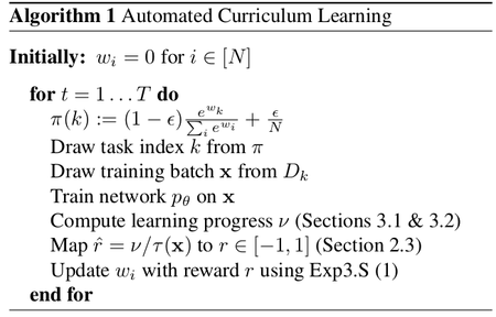
Algorithm

The automated curriculum learning is summarized as followed,

where $\tau(\mathbf{x})$ is the length of the longest input sequence. Since the processing time of each task may be different.

Fig 1. Automated Curriculum Learning Algorithm

Learning Progress Signals

The learning progress is the measurement of the effect of a training sample on the target objective. It usually is computationally undesirable or even impossible to obtain. Therefore the authors consider a range of signals derived from two distinct indicators of learning progress: 1) loss-driven, in the sense that they equate progress with a decrease in some loss; or 2) complexity-driven, when they equate progress with an increase in model complexity.

Loss-driven Progress

Five loss-driven progress signals are used and they compare the predictions made by the model before and after training on some sample $\mathbf{x}$.

Prediction gain(PG) Prediction gain is defined as the instantaneous change in loss for a sample $\mathbf{x}$ \[ v_{PG}:=L(\mathbf{x},\theta)-L(\mathbf{x},\theta') \]

Gradient prediction gain (GPG) This measures the magnitude of the gradient vector, which has been used an indicator of salience in the active learning samples \[ v_{GPG}:= || \triangledown L(\mathbf{x},\theta)||^2_2 \]

The above signals are instantaneous in the sense that they only depend on x. Such signals are appealing because they are typically cheaper to evaluate, and are agnostic about the overall goal of the curriculum. The remaining three signals more directly measure the effect of training on the desired objective but require an additional sample $x'$.

Self prediction gain (SPG) Self prediction gain samples a second time from the same task to address the bias problem of PG \[ v_{SPG}:=L(\mathbf{x}',\theta)-L(\mathbf{x}',\theta'), \quad \mathbf{x}' \sim D_k \]

Target prediction gain (TPG) \[ v_{TPG}:=L(\mathbf{x}',\theta)-L(\mathbf{x}',\theta'), \quad \mathbf{x}' \sim D_N \] Although this estimator might seem like the most accurate measure so far, it tends to suffer from high variance.

Mean prediction gain (MPG) \[ v_{MPG}:=L(\mathbf{x}',\theta)-L(\mathbf{x}',\theta'), \quad \mathbf{x}' \sim D_k, k \sim U_N, \] where $U_N$ denotes the uniform distribution on $\{1,\ldots,N\}$.

Complexity-driven Progress

The intuition for complexity gains is derived from the Minimum Description Length principle (Grunwald, 2007). It states that in order to achieve high generalization from a particular dataset, both the number of bits required to describe the model parameters and the data. This is of significance only if the increase in model complexity strongly reduces the data cost. In the case of neural networks, MDL training is done via stochastic variational inference ( Hinton and Van Camp 1993; Graves, 2011; Kingma et al., 2015; Blundell et al., 2015)

In the stochastic variational inference framework, a variational posterior $P_\phi(\theta)$ over the network weights is maintained during training, with a single weight sample drawn for each training example. An adaptive prior $Q_\psi(\theta)$ are reused for every network weight. In this paper, both of $P$ and $Q$ are set as a diagonal Gaussian distribution, such the complexity cost can be computed analytically \[ KL(P_\phi|| Q_\psi) = \frac{(\mu_\phi-\mu_\psi)^2+\sigma^2_\phi-\sigma^2_\psi}{２\sigma^2_\psi}+\ln\Big( \frac{\sigma_\psi}{\sigma_\phi} \Big) \]

Variational complexity gain (VCG) \[v_{VCG}:= KL(P_{\phi'}|| Q_{\psi'}) - KL(P_\phi|| Q_\psi)\]

Gradient variational complexity gain (GVCG) \[ v_{GVCG}:= [\triangledown_{\phi,\psi} KL(P_\phi|| Q_\psi)]^T \triangledown_\phi \mathbb{E}_{\theta \sim P_\phi}　　L(\mathbf{x},\theta) \]

L2 gain (L2G) \[ v_{L2G}:=|| \theta' ||^2_2 -|| \theta ||^2_2, \quad v_{GL2G}:=\theta^T [\triangledown_\theta L(\mathbf{x}, \theta)] \]

Experiments

To test the proposed approach, the authors applied all the gains to three tasks suites: $n$-gram models, repeat copy, and the bAbI tasks.

Unidirectional LSTM network architecture was used for all experiments, and cross-entropy was used as loss function. The neural network was optimized by RMSProp with momentum of $0.9$ and a learning rate $10^{-5}$. The parameters for Exp3S algorithm were $\eta = 10^{-3}, \beta = 0, \epsilon = 0.05$. All experiments were repeated $10$ times with different random initializations of network weights. Two performance benchmarks are 1) a fixed uniform policy over all the tasks and 2) directly training on the target task (where applicable).

N-Gram Language Modelling

The first experiment is the character-level KneserNey $n$-gram models (Kneser and Ney, 1995) on the King James Bible data from the Canterbury corpus, with the maximum depth parameter $n$ ranging between $0$ to $10$. It should be noticed that the amount of linguistic structure increases monotonically with $n$.

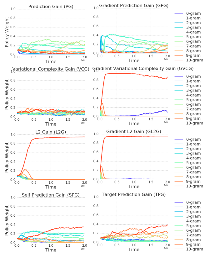
Fig. 2 shows that most of the complexity-based gain signals (L2G, GL2G, GVCG) progress rapidly through the curriculum before focusing strongly on the $10$-gram task. The loss-driven progress (PG, GPG, SPG, TG) also tend to move towards higher $n$, although more slowly and with less certainty. The authors note that the curriculum is unnecessary for this particular experiment. The 10-gram source was best learned by directly training on it. The loss based methods also favoured high n-grams for training but took longer to do so.

Fig 2. N-gram policies for different gain signals, truncated at $2 \times 10^8$ steps. All curves are averages over $10$ runs

Repeat Copy

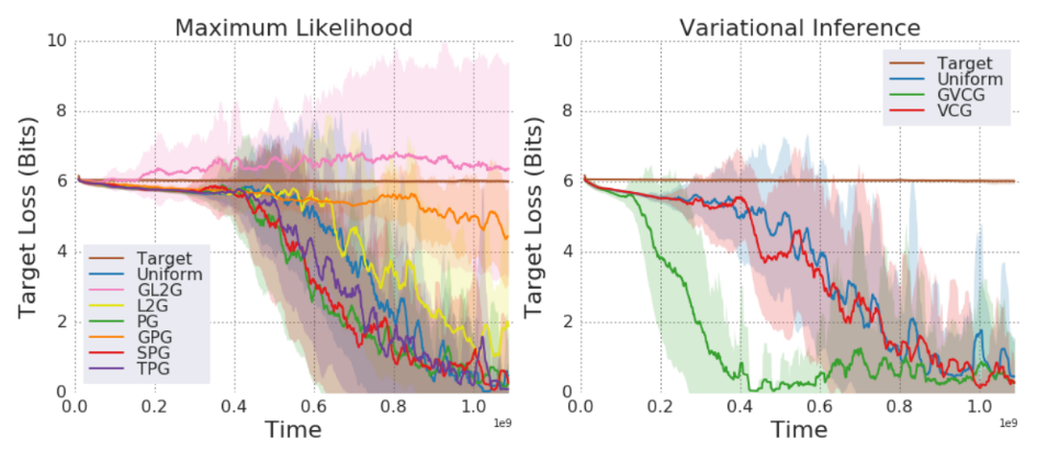
In the repeat copy task (Graves et al., 2014), the network is asked to repeat a random sequence a given number of times. Fig. 3 shows that GVCG solves the target task about twice as fast as uniform sampling for VI training, and that the PG, SPG and TPG gains are somewhat faster than uniform, especially in the early stages.

Fig 3. Target task loss (per output) truncated at $1.1 \times 10^9$ steps.. All curves are averages over $10$ runs

BAbI

The bAbI dataset (Weston et al., 2015) includes $20$ synthetic question-answering problems designed to test the basic reasoning capabilities of machine learning models. BAbI was not specifically designed for curriculum learning, but some of the tasks follow a natural ordering, such as ‘Two Arg Relations’, ‘Three Arg Relations’. The authors hope that an efficient syllabus could be found for learning the whole set.

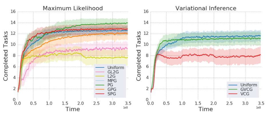
Fig. 4 shows that prediction gain (PG) clearly improved on uniform sampling in terms of both learning speed and number of tasks completed; for SPG the same benefits were visible, though less pronounced. The other gains were either roughly equal to or worse than uniform.

Fig 4. Completion curves for the bAbI curriculum, truncated at $3.5\times10^8$ steps. All curves are averages over $10$ runs

Conclusions

1. The experiments suggest that a stochastic syllabus can improve the significant gains when a suitable progress signal is used.

2. The uniform random task is a surprisingly strong benchmark. This is because learning is dominated by gradients from the tasks on which the network is making the fastest progress, thereby simulating a kind of implicit curriculum but with unnecessary samples.

3. The learning progress is best evaluated on a local, rather than global basis. In maximum likelihood training, prediction gain is the most consistent signal, while in variational inference training gradient variational complexity gain performed best.

Critique

In curriculum learning, a popular approach is to define a hand-chosen performance threshold for advancement to the next task, along with a fixed probability of returning to earlier tasks, to prevent forgetting. It is interesting to compare the performance of it and the proposed automated curriculum learning methods.

Here the assumption is that there is a pre-existing database with learning exemplars to sample from, but what if this isn't available? Forestier et al. tries to answer that problem.

Sources

• Graves, Alex, et al. "Automated Curriculum Learning for Neural Networks." arXiv preprint arXiv:1704.03003 (2017).
• Elman, Jeffrey L. "Learning and development in neural networks: The importance of starting small." Cognition 48.1 (1993): 71-99.
• Bengio, Yoshua, et al. "Curriculum learning." Proceedings of the 26th annual international conference on machine learning. ACM, 2009.
• Reed, Scott, and Nando De Freitas. "Neural programmer-interpreters." arXiv preprint arXiv:1511.06279 (2015).
• Gui, Liangke, Tadas Baltrušaitis, and Louis-Philippe Morency. "Curriculum Learning for Facial Expression Recognition." Automatic Face & Gesture Recognition (FG 2017), 2017 12th IEEE International Conference on. IEEE, 2017.
• Zaremba, Wojciech, and Ilya Sutskever. "Learning to execute." arXiv preprint arXiv:1410.4615 (2014).
• Kneser, Reinhard, and Hermann Ney. "Improved backing-off for m-gram language modeling." Acoustics, Speech, and Signal Processing, 1995. ICASSP-95., 1995 International Conference on. Vol. 1. IEEE, 1995.
• Weston, Jason, et al. "Towards ai-complete question answering: A set of prerequisite toy tasks." arXiv preprint arXiv:1502.05698 (2015).
• Graves, Alex, Greg Wayne, and Ivo Danihelka. "Neural turing machines." arXiv preprint arXiv:1410.5401 (2014).
• Grunwald, P. D. (2007). The minimum description length principle. The MIT Press.
• Hinton, G. E. and Van Camp, D. (1993). Keeping the neural networks simple by minimizing the description length of the weights. In Proceedings of the sixth annual conference on Computational learning theory, pages 5–13. ACM
• Sébastien Forestier1, Yoan Mollard, Intrinsically Motivated Goal Exploration Processes with Automatic Curriculum Learning
• Blundell, C., Cornebise, J., Kavukcuoglu, K., and Wierstra, D. (2015). Weight uncertainty in neural networks. In Proceedings of The 32nd International Conference on Machine Learning, pages 1613–1622
• Kingma, D. P., Salimans, T., and Welling, M. (2015). Variational dropout and the local reparameterization trick. In Advances in Neural Information Processing Systems, pages 2575–2583