Deep Exploration via Bootstrapped DQN: Difference between revisions
No edit summary |
|||
| Line 350: | Line 350: | ||
==B Bootstrapped DQN implementation== | ==B Bootstrapped DQN implementation== | ||
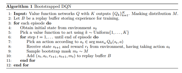
[[File: | [[File: alg1.PNG]] | ||
Revision as of 17:59, 20 November 2017
Details
Title: Deep Exploration via Bootstrapped DQN
Authors: Ian Osband {1,2}, Charles Blundell {2}, Alexander Pritzel {2}, Benjamin Van Roy {1}
Organisations:
- Stanford University
- Google Deepmind
Conference: NIPS 2016
URL: papers.nips.cc
Online code sources
This summary contains background knowledge from Section 2-7 (except Section 5). Feel free to skip if you already know.
Intro to Reinforcement Learning
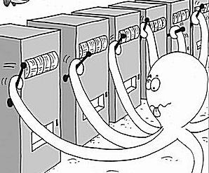
In reinforcement learning, an agent interacts with an environment with the goal to maximize its long term reward. A common application of reinforcement learning is to the multi armed bandit problem. In a multi armed bandit problem, there is a gambler and there are $n$ slot machines, and the gambler can choose to play any specific slot machine at any time. All the slot machines have their own probability distributions by which they churn out rewards, but this is unknown to the gambler. So the question is, how can the gambler learn how to get the maximum long term reward?
There are two things the gambler can do at any instance: either he can try a new slot machine, or he can play the slot machine he has tried before (and he knows he will get some reward). However, even though trying a new slot machine feels like it would bring less reward to the gambler, it is possible that the gambler finds out a new slot machine that gives a better reward than the current best slot machine. This is the dilemma of exploration vs exploitation. Trying out a new slot machine is exploration, while redoing the best move so far is exploiting the currently understood perception of the reward.
There are many strategies to approach this exploration-exploitation dilemma. Some common strategies for optimizing in an exploration-exploitation setting are Random Walk, Curiosity-Driven Exploration, and Thompson Sampling. A lot of these approaches are provably efficient, but assume that the state space is not very large. For instance, the approach called Curiosity-Driven Exploration aims to take actions that lead to immediate additional information. This requires the model to search “every possible cell in the grid” which is not desirable if state space is very large. Strategies for large state spaces often just either ignore exploration, or do something naive like $\epsilon$-greedy, where you exploit with $1-\epsilon$ probability and explore "randomly" in rest of the cases.
This paper tries to use a Thompson sampling like approach to make decisions.
Thompson Sampling[1]
In Thompson sampling, our goal is to reach a belief that resembles the truth. Let's consider a case of coin tosses (2-armed bandit). Suppose we want to be able to reach a satisfactory pdf for $\mathbb{P}_h$ (heads). Assuming that this is a Bernoulli bandit problem, i.e. the rewards are $0$ or $1$, we can start off with $\mathbb{P}_h^{(0)}=\beta(1,1)$. The $\beta(x,y)$ distribution is a very good choice for a possible pdf because it works well for Bernoulli rewards. Further $\beta(1,1)$ is the uniform distribution $\mathbb{N}(0,1)$.
Now, at every iteration $t$, we observe the reward $R^{(t)}$ and try to make our belief close to the truth by doing a Bayesian computation. Assuming $p$ is the probability of getting a heads,
$$ \begin{align*} \mathbb{P}(R|D) &\propto \mathbb{P}(D|R) \cdot \mathbb{P}(R) \\ \mathbb{P}_h^{(t+1)}&\propto \mbox{likelihood}\cdot\mbox{prior} \\ &\propto p^{R^{(t)}}(1-p)^{R^{(t)}} \cdot \mathbb{P}_h^{(t)} \\ &\propto p^{R^{(t)}}(1-p)^{R^{(t)}} \cdot \beta(x_t, y_t) \\ &\propto p^{R^{(t)}}(1-p)^{R^{(t)}} \cdot p^{x_t-1}(1-p)^{y_t-1} \\ &\propto p^{x_t+R^{(t)}-1}(1-p)^{y_t+R^{(t)}-1} \\ &\propto \beta(x_t+R^{(t)}, y_t+R^{(t)}) \end{align*} $$
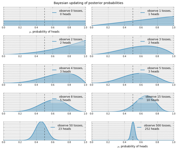
This means that with successive sampling, our belief can become better at approximating the truth. There are similar update rules if we use a non Bernoulli setting, say, Gaussian. In the Gaussian case, we start with $\mathbb{P}_h^{(0)}=\mathbb{N}(0,1)$ and given that $\mathbb{P}_h^{(t)}\propto\mathbb{N}(\mu, \sigma)$ it is possible to show that the update rule looks like
$$ \mathbb{P}_h^{(t+1)} \propto \mathbb{N}\bigg(\frac{t\mu+R^{(t)}}{t+1},\frac{\sigma}{\sigma+1}\bigg) $$
How can we use this in reinforcement learning?
We can use this idea to decide when to explore and when to exploit. We start with an initial belief, choose an action, observe the reward and based on the kind of reward, we update our belief about what action to choose next.
Bootstrapping [2,3]
This idea may be unfamiliar to some people, so I thought it would be a good idea to include this. In statistics, bootstrapping is a method to generate new samples from a given sample. Suppose that we have a given population, and we want to study a measure $\theta$. So, we just find $n$ sample points (sample $\{D_i\}_{i=1}^n$), calculate this measure $\hat{\theta}$ for these $n$ points, and make our inference.
If we later wish to find a better bound on $\hat{\theta}$, i.e. suppose we want to say that $\delta_1 \leq \hat{\theta} \leq \delta_2$ with a confidence of $c$, then we can use bootstrapping for this.
Using bootstrapping, we can create a new sample $\{D'_i\}_{i=1}^{n'}$ by randomly sampling $n'$ times from $D$, with replacement. So, if $D=\{1,2,3,4\}$, a $D'$ of size $n'=10$ could be $\{1,4,4,3,2,2,2,1,3,4\}$. We do this a sufficient $k$ number of times, calculate $\hat{\theta}$ each time, and thus get a distribution $\{\hat{\theta}_i\}_{i=1}^k$. Now, we can choose the $100\cdot c$th and $100\cdot(1-c)$th percentile of this distribution, (let them be $\hat{\theta}_\alpha$ and $\hat{\theta}_\beta$ respectively) and say
$$\hat{\theta}_\alpha \leq \hat{\theta} \leq \hat{\theta}_\beta, \mbox{with confidence }c$$
Why choose bootstrap and not dropout?
There is previous work[4] that establishes dropout as a good way to train NNs on a posterior such that the trained NN works like a function approximator that is close to the actual posterior. But, there are several problems with the predictions of this trained NN. The figures below are from the appendix of this paper. The left image is the NN trained by the authors of this paper on a sample noisy distribution and the right image is from the accompanying web demo from [4], where the authors of [4] show that their NN converges around the mean with a good confidence.

According to the authors of this paper,
- Even though [4] says that dropout converges arond the mean, their experiment actually behaves weirdly around a reasonable point like $x=0.75$. They think that this happens because dropout only affects the region local to the original data.
- Samples from the NN trained on the original data do not look like a reasonable posterior (very spiky).
- The trained NN collapses to zero uncertainty at the data points from the original data.
Q Learning and Deep Q Networks [5]
At any point of time, our rewards dictate what our actions should be. Also, in general, we want good long term rewards. For example, if we are playing a first person shooter game, it is a good idea to go out of cover to kill an enemy, even if some health is lost. Similarly, in reinforcement learning, we want to maximize our long term reward. So if at each time $t$, the reward is $r_t$, then a naive way is to say we want to maximise
$$ R_t = \sum_{i=0}^{\infty}r_t $$
But, this reward is unbounded. So technically it could tend to $\infty$ in a lot of the cases. This is why we use a discounted reward.
$$ R_t = \sum_{i=0}^{\infty}\gamma^t r_t $$
Here, we take $0\leq \gamma \lt 1$. So, what this means is that we value our current reward the most ($r_0$ has a coefficient of $1$), but we also consider the future possible rewards. So if we had two choices: get $+4$ now and $0$ at all other timesteps, or get $-2$ now and $+2$ after $3$ timesteps for $20$ timesteps, we choose the latter ($\gamma=0.9$). This is because $(+4) < (-2)+0.9^3(2+0.9\cdot2+\cdots+0.9^{19}\cdot2)$.
A policy $\pi: \mathbb{S} \rightarrow \mathbb{A}$ is just a function that tells us what action to take in a given state $s\in \mathbb{S}$. Our goal is to find the best policy $\pi^*$ that maximises the reward from a given state $s$. So, a value function is defined from $s$ (which the agent is in, at timestep $t$) and following the policy $\pi$ as $V^\pi(s) = \mathbb{E}[R_t]$. The optimal value function is then simply
$$ V^*(s)=\displaystyle\max_{\pi}V^\pi(s) $$
For convenience however, it is better to work with the Q function $Q: \mathbb{S}\times\mathbb{A} \rightarrow \mathbb{R}$. $Q$ is defined similarly as $V$. It is the expected return after taking an action $a$ in the given state $s$. So, $Q^\pi(s,a)=\mathbb{E}[R_t|s,a]$. The optimal $Q$ function is
$$ Q^*(s,a)=\displaystyle\max_{\pi}Q^\pi(s,a) $$
Suppose that we know $Q^*$. Then, if we know that we are supposed to start at $s$ and take an action $a$ right now, what is the best course of action from the next time step? We just choose the optimal action $a'$ at the next state $s'$ that we reach. The optimal action $a'$ at state $s'$ is simply the argument $a_x$ that maximises our $Q^*(s',\cdot)$.
$$ a'=\displaystyle\arg\max_{a_x} Q^*(s',a_x) $$
So, our best expected reward from $s$ taking action $a$ is $\mathbb{E}[r_t+\gamma\mathbb{E}[R_{t+1}]]$. This is known as the Bellman equation:
$$ Q^*(s,a)=\mathbb{E}[r_t+\gamma \displaystyle\arg\max_{a_x} Q^*(s',a_x)] $$
In Q learning, we use a deep neural network with weights $\theta$ as a function approximator for $Q^*$. The naive way to do this is to design a deep neural net that takes as input the state $s$ and action $a$, and produces an approximation to $Q^*$.
- Suppose our neural net weights are $\theta_i$ at iteration $i$.
- We want to train our neural net on the case when we are at $s$, take action $a$, get reward $r$, and reach $s'$.
- To find out what action is best from $s'$, i.e. $a'$, we have to simulate all actions from $s'$. We can do this after we complete this iteration, then run $s',a_x$ for all $a_x\in\mathbb{A}$. But, we don't know how to complete this iteration without knowing this $a'$. So, another way is to simulate all actions from $s'$ using last known set of weights $\theta_{i-1}$. We just simulate state $s'$, action $a_x$ for all $a_x\in\mathbb{A}$ from the previous state and get $Q^*(s',a_x;\theta_{i-1})$. (Note that some papers do not use the set of weights from the previous iteration $\theta_{i-1}$. Instead they fix the weights for finding the best action for every $\tau$ steps to $\theta^-$, and do $Q^*(s',a_x;\theta^-)$ for $a_x\in\mathbb{A}$ and use this for the target value.)
- Now we can compute our loss function using the Bellman equation, and backpropagate.
$$ \mbox{loss}=\mbox{target}-\mbox{prediction}=(r+\displaystyle\max_{a_x}Q^*(s',a_x;\theta_{i-1}))-Q^*(s,a;\theta_i) $$
The problem with this approach is that at every iteration $i$, we have to do $|\mathbb{A}|$ forward passes on the previous set of weights $\theta_{i-1}$ to find out the best action $a'$ at $s'$. This becomes infeasible quickly with more possible actions.
Authors of [5] therefore use another kind of architecture. This architecture takes as input the state $s$, and computes the values $Q^*(s,a_x)$ for $a_x\in\mathbb{A}$. So there are $|\mathbb{A}|$ outputs. This basically parallelizes the forward passes so that $r+\displaystyle\max_{a_x}Q^*(s',a_x;\theta_{i-1})$ can be done with just a single pass through the outputs.
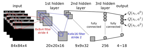
Note: When I say state $s$ as an input, I mean some representation of $s$. Since the environment is a partially observable MDP, it is hard to know $s$. So, we can for example, apply a convnet on the frames and get an idea of what the current state is. We pass this output to the input of the DNN (DNN is the fully connected layer for the convnet then).
Experience Replay
Authors of this paper borrow the concept of experience replay from [5,6]. In experience replay, we do training in episodes. In each episode, we play and store consecutive $(s,a,r,s')$ tuples in the experience replay buffer. Then after the play, we choose random samples from this buffer and do our training.
Advantages of experience replay over simple online Q learning[5]:
- Better data efficiency: It is better to use one transition many times to learn again and again, rather than just learn once from it.
- Learning from consecutive samples is difficult because of correlated data. Experience replay breaks this correlation.
- Online learning means the input is decided by the previous action. So, if the maximising action is to go left in some game, next inputs would be about what happens when we go left. This can cause the optimiser to get stuck in a feedback loop, or even diverge, as [7] points out.
Double Q Learning
Problem with Q Learning[8]
For a simple neural network, each update tries to shift the current $Q^*$ estimate to a new value:
$$ Q^*(s,a) \leftarrow r+\gamma\displaystyle\max_{a_x}Q^*(s',a_x) $$
Suppose the neural net has some inherent noise $\epsilon$. So, the neural net actually stores a value $\mathbb{Q}^*$ given by
$$ \mathbb{Q}^* = Q^*+\epsilon $$
Even if $\epsilon$ has zero mean in the beginning, using the $\max$ operator at the update steps will start propagating $\gamma\cdot\max \mathbb{Q}^*$. This leads to a non zero mean subsequently. The problem is that "max causes overestimation because it does not preserve the zero-mean property of the errors of its operands." ([8]) Thus, Q learning is more likely to choose overoptimistic values.
How does Double Q Learning work? [9]
The problem can be solved by using two sets of weights $\theta$ and $\Theta$. The $\mbox{target}$ can be broken up as
$$ \mbox{target} = r+\displaystyle\max_{a_x}Q^*(s',a_x;\theta) = r+Q^*(s',\displaystyle\arg\max_{a_x}Q^*(s',a_x;\theta);\theta) = r+Q^*(s',a';\theta) $$
Using double Q learning, we select the best action using current weights $\theta$ and evaluate the $Q^*$ value to decide the target value using $\Theta$.
$$ \mbox{target} = r+Q^*(s',\displaystyle\arg\max_{a_x}Q^*(s',a_x;\theta);\Theta) = r+Q^*(s',a';\Theta) $$
This makes the evaluation fairer.
Double Deep Q Learning
[9] further talks about how to use this for deep learning without much additional overhead. The suggestion is to use $\theta^-$ as $\Theta$.
$$ \mbox{target} = r+Q^*(s',\displaystyle\arg\max_{a_x}Q^*(s',a_x;\theta);\theta^-) = r+Q^*(s',a';\theta^-) $$
Bootstrapped DQN
The authors propose an architecture that has a shared network and $K$ bootstrap heads. So, suppose our experience buffer $E$ has $n$ datapoints, where each datapoint is a $(s,a,r,s')$ tuple. Each bootstrap head trains on a different buffer $E_i$, where each $E_i$ has been constructed by sampling $n$ datapoints from the original experience buffer $E$ with replacement (bootstrap method).
Because each of the heads train on a different buffer, they model a different $Q^*$ function (say $Q^*_k$). Now, for each episode, we first choose a specific $Q^*_k=Q^*_s$. This $Q^*_s$ helps us create the experience buffer for the episode. From any state $s_t$, we populate the experience buffer by choosing the next action $a_t$ that maximises $Q^*_s$. (similar to Thompson Sampling)
$$ a_t = \displaystyle\arg\max_a Q^*_s(s_t,a_t) $$
Also, along with $s_t,a_t,r_t,s_{t+1}$, they push a bootstrap mask $m_t$. This mask is basically is a binary vector of size $K$, and it tells which $Q_k$ should be affected by this datapoint, if it is chosen as a training point. So, for example, if $K=5$ and there is a experience tuple $(s_t,a_t,r_t,s_{t+1},m_t)$ where $m_t=(0,1,1,0,1)$, then $(s_t,a_t,r_t,s_{t+1})$ should only affect $Q_2,Q_3$ and $Q_5$.
So, at each iteration, we just choose few points from this buffer and train the respective $Q_{(\cdot)}$ based on the bootstrap masks.
How to generate masks?
Masks are created by sampling from the masking distribution. Now, there are many ways to choose this masking distribution:
- If for each datapoint $D_i$ ($i=1$ to $n$), we mask from $\mbox{Bernoulli}(0.5)$, this will roughly allow us to have half the points from the original buffer. To get to size $n$, we duplicate these points by doubling the weights for each datapoint. This essentially gives us a double or nothing bootstrap[10].
- If the mask is $(1, 1 \cdots 1)$, then this becomes an ensemble learning method.
- $m_t~\mbox{Poi}(1)$ (poisson distribution)
- $m_t[k]~\mbox{Exp}(1)$ (exponential distribution)
For this paper's results, the authors used a $\mbox{Bernoulli}(p)$ distribution.
Related Work
The authors mention the method described in [11]. The authors of [11] talk about the principle of "optimism in the face of uncertainty" and modify the reward function to encourage state-action pairs that have not been seen often:
$$ R(s,a) \leftarrow R(s,a)+\beta\cdot\mbox{novelty}(s,a) $$
According to the authors, [11]'s DQN algorithm relies on a lot of hand tuning and is only good for non stochastic problems. The authors further compare their results to [11]'s results on Atari.
The authors also mention an existing algorithm PSRL[12,13], or posterior sampling based RL. However, this algorithm requires a solved MDP, which is not feasible for large systems. Bootstrapped DQN approximates this idea by sampling from approximate $Q^*$ functions.
Further, the authors mention that the work in [12,13] has been followed by RLSVI[14] which solves the problem for linear cases.
Deep Exploration: Why is Bootstrapped DQN so good at it?
The authors consider a simple example to demonstrate the effectiveness of bootstrapped DQN at deep exploration.

In this example, the agent starts at $s_2$. There are $N$ steps, and $N+9$ timesteps to generate the experience buffer. The agent is said to have learned the optimal policy if it achieves the best possible reward of $10$ (go to the rightmost state in $N-1$ timesteps, then stay there for $10$ timesteps), for at least $100$ such episodes. The results they got:

The blue dots indicate when the agent learnt the optimal policy. If this took more than $2000$ episodes, they indicate it with a red dot. Thompson DQN is DQN with posterior sampling at every timestep. Ensemble DQN is same as bootstrapped DQN except that the mask is all $(1,1 \cdots 1)$. It is evident from the graphs that bootstrapped DQN can achieve deep exploration better than these two methods, and DQN.
But why is it better?
The authors say that this is because bootstrapped DQN constructs different approximations to the posterior $Q^*$ with the same initial data. This diversity of approximations is because of random initalization of weights for the $Q^*_k$ heads. This means that these heads start out trying random actions (because of diverse random initial $Q^*_k$), but when some head finds a good state and generalises to it, some (but not all) of the heads will learn from it, because of the bootstrapping. Eventually other heads will either find other good states, or end up learning the best good states found by the other heads.
So, the architecture explores well and once a head achieves the optimal policy, eventually, all heads achieve the policy.
Results
The authors test their architecture on 49 Atari games. They mention that there has been recent work to improve the performance of DDQNs, but those are tweaks whose intentions are orthogonal to this paper's idea. So, they don't compare their results with them.
Scale: What values of $K$, $p$ are best?

Recall that $K$ is the number of bootstrap heads and $p$ is the parameter for the masking distribution (Bernoulli). The authors say that around $K=10$, the performance reaches close to the peak, so it should be good.
$p$ also represents the amount of data sharing. This is because lesser $p$ means there is lesser chance (due to the Bernoulli distribution) that the corresponding datapoint is taken into the bootstrapped dataset $D_i$. So, lesser $p$ means more identical datapoints, hence more heads share their datapoints. However, the value of $p$ doesn't seem to affect the rewards achieved over time. The authors give the following reasons for it:
- The heads start with random weights for $Q^*$, so the targets (which use $Q^*$) turn out to be different. So the update rules are different.
- Atari is deterministic.
- Because of the initial diversity, the heads will learn differently even if they predict the same action for the given state.
$p=1$ is the value they use finally, because this reduces the no. of identical datapoints and reduces time.
Performance on Atari
In general, the results tell us that bootstrapped DQN achieves better results.
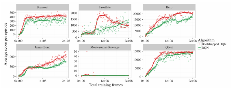
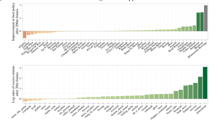
The authors plot the improvement they achieved with bootstrapped DQN with the games. They define improvement to be $x$ if bootstrapped DQN achieves a better result than DQN in $\frac{1}{x}$ frames.

The authors say that bootstrapped DQN doesn't work good on all Atari games. They point out that there are some challenging games, where exploration is key but bootstrapped DQN doesn't do good enough (but does better than DQN). Some of these games are Frostbite and Montezuma’s Revenge. They say that even better exploration may help, but also point out that there may be other problems like: network instability, reward clipping and temporally extended rewards.
Improvement: Highest Score Reached & how fast is this high score reached?
The authors plot the improvement graphs after 20m and 200m frames.
Visualisation of Results
One of the authors' youtube playlist can be found online.
The authors also point out that just purely using bootstrapped DQN as an exploitative strategy is pretty good by itself, better than vanilla DQN. This is because of the deep exploration capabilities of bootstrapped DQN, since it can use the best states it knows and also plan to try out states it doesn't have any information about. Even in the videos, it can be seen that the heads agree at all the crucial decisions, but stay diverse at other less important steps.
Critique
It would be very interesting and a great addition to the the experimental section of the paper, if the authors would have compared with asynchronous methods of exploration of the state space first introduced in [15]. The authors unfortunately only compared their DQN with the original DQN and not all the other variations in the literature, and justified it by saying that their idea was "orthogonal" to these improvements.
Different way to do exploration-exploitation?
Instead of choosing the next action $a_t$ that maximises $Q^*_s$, they could have chosen different actions $a_i$ with probabilities
$$ \mathbb{P}(s_t,a_i) = \frac{Q^*_s(s_t,a_i)}{\displaystyle \sum_{i=1}^{|\mathbb{A}|} Q^*_s(s_t,a_i)} $$
According to me, this is closer to Thompson Sampling.
Why use Bernoulli?
The choice of having a Bernoulli masking distribution eventually doesn't help them at all, since the algorithm does good because of the initial diversity. Maybe they can use some other masking distribution?
Unanswered Questions & Miscellaneous
- Why does Thompson DQN perform poorly?
- The actual algorithm is hidden in the appendix. It could have been helpful if it were in the main paper.
References
- Learning and optimization for sequential decision making, Columbia University, Lec 4
- Thoughtco, What is bootstrapping in statistics?
- Bootstrap confidence intervals, Class 24, 18.05, MIT Open Courseware
- Yarin Gal and Zoubin Ghahramani. Dropout as a bayesian approximation: Representing model uncertainty in deep learning. arXiv preprint arXiv:1506.02142, 2015.
- Mnih et al., Playing Atari with Deep Reinforcement Learning, 2015
- Long-Ji Lin. Reinforcement learning for robots using neural networks. Technical report, DTIC Document, 1993.
- John N Tsitsiklis and Benjamin Van Roy. An analysis of temporal-difference learning with function approximation. Automatic Control, IEEE Transactions on, 42(5):674–690, 1997.
- S. Thrun and A. Schwartz. Issues in using function approximation for reinforcement learning, 1993.
- Hado Van Hasselt, Arthur Guez, and David Silver. Deep reinforcement learning with double q-learning, 2015.
- Dean Eckles and Maurits Kaptein, Thompson Sampling with the Online Bootstrap, 2014, Pg 3
- Bradly C. Stadie, Sergey Levine, Pieter Abbeel, Incentivizing Exploration In Reinforcement Learning With Deep Predictive Models, 2015.
- Ian Osband, Daniel Russo, and Benjamin Van Roy. (More) efficient reinforcement learning via posterior sampling, NIPS 2013.
- Ian Osband and Benjamin Van Roy. Model-based reinforcement learning and the eluder dimension, NIPS 2014.
- Ian Osband, Benjamin Van Roy, Zheng Wen, Generalization and Exploration via Randomized Value Functions, 2014.
- Mnih, Volodymyr, et al. "Asynchronous methods for deep reinforcement learning." International Conference on Machine Learning. 2016.
Other helpful links (unsorted):
