Convolutional Sequence to Sequence Learning

Introduction

Sequence to sequence learning has been used to solve many tasks such as machine translation, speech recognition and text summarization. Most of the past models employ RNNs for this problem, with bidirectional RNNs with soft attention being the dominant approach. On the other hand, CNNs have not been used for this task, despite the many advantages they offer:

• Compared to recurrent layers, convolutions create representations for fixed size contexts, however, the effective context size of the network can easily be made larger by stacking several layers on top of each other. This allows to precisely control the maximum length of dependencies to be modeled.
• Convolutional networks do not depend on the computations of the previous time step and therefore allow parallelization over every element in a sequence. This contrasts with RNNs which maintain a hidden state of the entire past that prevents parallel computation within a sequence.
• Multi-layer convolutional neural networks create hierarchical representations over the input sequence in which nearby input elements interact at lower layers while distant elements interact at higher layers. This provides a shorter path to capture long-range dependencies compared to the chain structure modeled by recurrent networks.

In this paper, the authors introduce an architecture for sequence learning based entirely on convolutional neural networks. Compared to recurrent models, computations over all elements can be fully parallelized during training to better exploit the GPU hardware and optimization is easier since the number of non-linearities is fixed and independent of the input length. The use of gated linear units eases gradient propagation and equipping each decoder layer with a separate attention module adding a negligible amount of overhead. The combination of these choices enables to tackle large scale problems. They outperform the accuracy of the deep LSTM setup of Wu et al. (2016) and is now the state of the art model for neural machine translation.

Related Work

Bradbury et al.(2016) introduce a quasi-recurrent neural network (QRNNs), an approach to neural sequence modelling that alternates convolutional layers, which apply in parallel across timesteps, and a minimalist recurrent pooling function that applies in parallel across channels. They use QRNNs for sentiment classification, language modelling and aslo briefly describe about an architecture consisting of QRNNs for sequence to sequence learning.

Kalchbrenner et al.(2016) introduce an architecture called "bytenet". The ByteNet is a one-dimensional convolutional neural network that is composed of two parts, one to encode the source sequence and the other to decode the target sequence. This network has two core properties: it runs in time that is linear in the length of the sequences and it sidesteps the need for excessive memorization.

However, none of the above approaches has been demonstrated improvements over state of the art results on large benchmark datasets. Gated convolutions have been previously explored for machine translation by Meng et al. (2015) but their evaluation was restricted to a small dataset. The author himself has explored architectures which used CNN but only in the encoder, the decoder part was still Recurrent.

Background

• Sequence to sequence Learning with RNNs - https://wiki.math.uwaterloo.ca/statwiki/index.php?title=stat946f15/Sequence_to_sequence_learning_with_neural_networks
• Perplexity(PPL) - In machine learning, the term perplexity has three closely related meanings. Perplexity is a measure of how easy a probability distribution is to predict. Perplexity is a measure of how variable a prediction model is. And perplexity is a measure of prediction error. The third meaning of perplexity is calculated slightly differently but all three have the same fundamental idea. This is given by [math]\displaystyle{ 2^{{H(p)}}=2^{{-\sum _{x}p(x)\log _{2}p(x)}} }[/math] Suppose you have a four-sided dice (not sure what that’d be). The dice is fair so all sides are equally likely (0.25, 0.25, 0.25, 0.25) and so it’s value here is 4.00. Now suppose you have a different dice whose sides have probabilities (0.10, 0.40, 0.20, 0.30). This dice has perplexity 3.5961 which is lower than 4.00 because it’s easier to predict (namely, predict the side that has p = 0.40).

• BLEU (BiLingual Evaluation Understudy) - It is an algorithm for evaluating the quality of text which has been machine-translated from one natural language to another. Quality is considered to be the correspondence between a machine's output and that of a human: "the closer a machine translation is to a professional human translation, the better it is" – this is the central idea behind BLEU. Additionally, it was one of the first metrics to claim a high correlation with human judgements of quality [11, 12 and 13] and remains one of the most popular automated and inexpensive metrics. More details at : http://www1.cs.columbia.edu/nlp/sgd/bleu.pdf

• Gating Mechanisms Gating mechanisms control information flow within a neural network. For example, LSTMs use gating mechanisms to enable long-term memory by using a separate cell controlled by input and forget gates. These gates prevent information from vanishing through transformations. CNNs are not limited by vanishing gradients and do not require forget gates as LSTMs. Gates are useful in controlling what information is propagated through a hierarchy of layers.

Convolutional Architecture

Position Embeddings

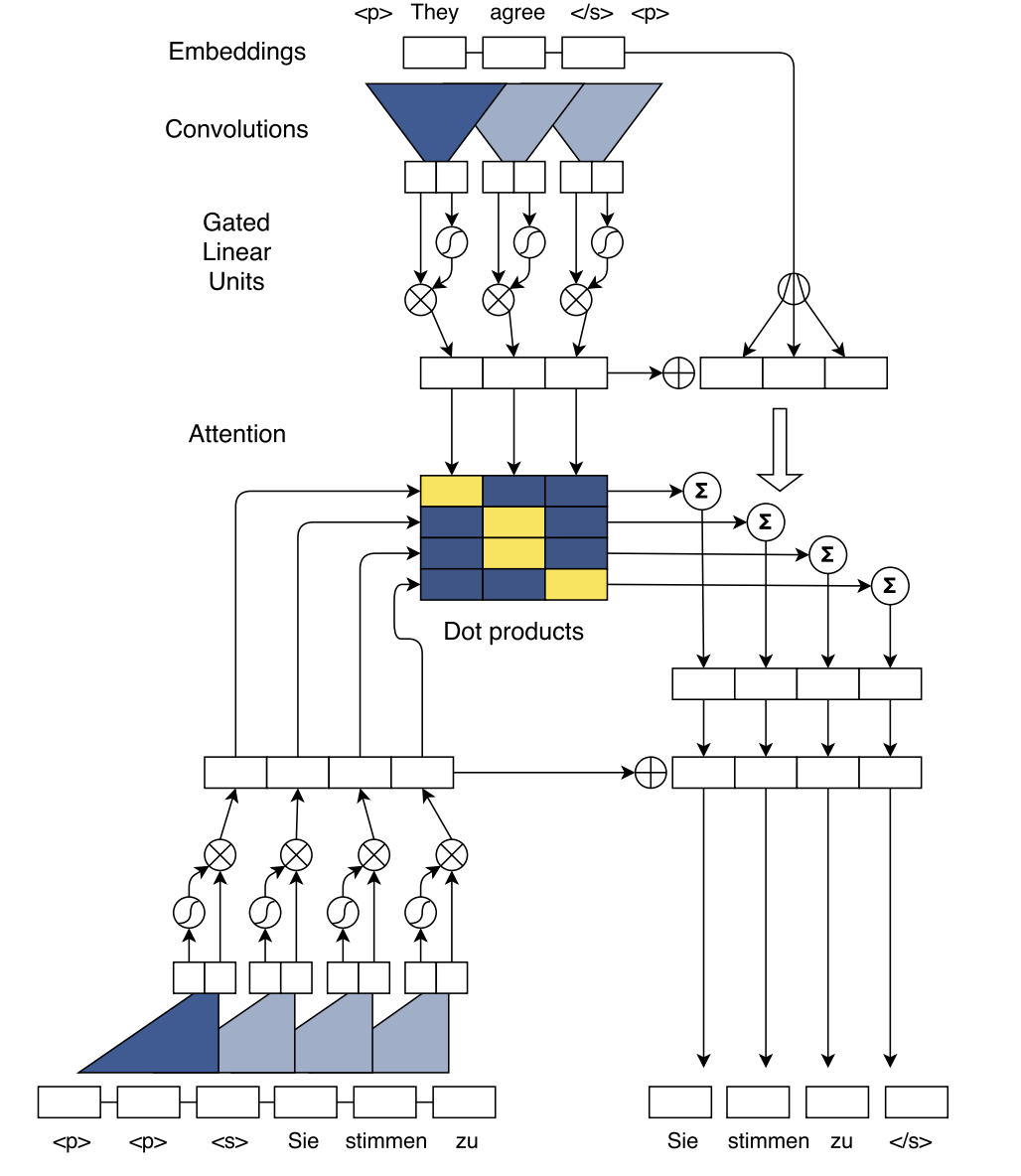
The architecture uses both word embeddings as well as positional embeddings as the input for the Convolutional Layer. The position order is used to equip the model to recognize the ordering of the word in the sequence and helps the model to know which element it is dealing with.

For input words [math]\displaystyle{ x = (x_1, ...,x_m) }[/math] we get the word vector representation as [math]\displaystyle{ w = (w_1,....,w_m) }[/math] and position vectors as [math]\displaystyle{ p = (p_1,....,p_m) }[/math] where [math]\displaystyle{ p_i }[/math] denotes the actual position of the word in the input sequence.

Both the vectors are combined to get the input element representation [math]\displaystyle{ e = (w_1 + p_1,....,w_m+p_m) }[/math]

Similarly for output elements that were already generated by the decoder network to yield output element representations that are being fed back into the decoder network [math]\displaystyle{ g = (g_1,....,g_n) }[/math]

Convolutional Block Structure

Both encoder and decoder networks share a simple structure of blocks/layers that computes intermediate states based on a fixed number of input elements. The output of l-th block of decoder is denoted by [math]\displaystyle{ h^l = (h_1^l,....,h_n^l) }[/math] and [math]\displaystyle{ z^l = (z_1^l,....,z_m^l) }[/math]. Each block contains a one-dimensional convolution followed by a non-linearity. For a decoder network with a single block and kernel width k, each resulting state [math]\displaystyle{ h_i^1 }[/math] contains information over k input elements. Stacking several blocks on top of each other increases the number of input elements represented in a state. For instance, stacking 6 blocks with k = 5 results in an input field of 25 elements or we can also say that output depends on 25 input elements.

A kernal parameters is represented as [math]\displaystyle{ W ∈ ℝ^{2d x kd}, b_w ∈ ℝ^{2d} }[/math] and takes as input [math]\displaystyle{ X ∈ ℝ^{k×d} }[/math] to produce output element [math]\displaystyle{ Y ∈ ℝ^{2d} }[/math]. The non linearity chosen was Gated Linear Unit(GLU) mainly because it was shown to perform better in aspects of langauge modelling. A GLU produes an output [math]\displaystyle{ v([A B]) = A ⊗ σ(B), v([AB]) ∈ ℝ^{d} }[/math] and [math]\displaystyle{ Y = [AB] ∈ ℝ^{2d} }[/math].

A residual connection is added from the input of each block to the output of each block. This is done so that the model can be deep. He et al. (Deep Residual Learning for Image Recognition) showed that adding residual connections improve the model performance by making it deep and prevents degradation of training accuracy. This is given by the equation [math]\displaystyle{ h_i^l = v(W^l [h_{i-k/2}^{l-1},...,h_{i+k/2}^{l-1}] + b_w^l) + h_i^{l-1} }[/math]

Padding is performed in the encoder after the convolution step so that the output matches the length of the input. The same cannot be applied to the decoder as we don't know the size of the sequence. To overcome this they pad the input of decoder with k-1 zeroes on both the left and right side and then prune the last k elements from the convolutional output. They add a linear mapping to project between embedding size [math]\displaystyle{ f }[/math] and convolutional output of size 2d. They apply such a transform to w when feeding embeddings to the encoder network, to the encoder output [math]\displaystyle{ z_j^u }[/math], to the final layer of the decoder just before the softmax [math]\displaystyle{ h^l }[/math], and to all decoder layers [math]\displaystyle{ h^l }[/math] before computing attention scores.

Finally, a probability distribution is generated over next T possible candidates elements [math]\displaystyle{ p(y_{i+1} | y_i,...y_1,x) = softmax(W_o h_i^l + b_o) ∈ ℝ^T }[/math]

Multi-step Attention

A separate attention mechanism is used for each decoder block. To compute the attention decoder state of current layer is combined with the embedding of the last element generated [math]\displaystyle{ g_i }[/math] we can now write state summary as [math]\displaystyle{ d_i^l = W_d^l + b_i^l + g_i }[/math]. For a decoder layer l the attention [math]\displaystyle{ a_{ij}^l }[/math] with state i and source element j is computed as [math]\displaystyle{ a_{ij}^l = \frac{exp(d_i^l . z_j^u)}{\sum_{t=1}^m exp(d_i^l . z_t^u)} }[/math]. The conditional input to the decoder layer is weighted sum of encoder and element embeddings. This can be written as [math]\displaystyle{ c_i^l = \sum_{j=1}^m a_{i,j}^l (z_j^u + e_j) }[/math]. This conditional input is then added to the decoder state [math]\displaystyle{ h_i^l }[/math],

The attention in the first layer provides the source context which is then fed to the next layer which takes this information to compute other information in that layer. The decoder aslo has the history of previous attention as [math]\displaystyle{ h_i^l = h_i^l + c_i^l }[/math]

Normalization Strategy and initialization

They use Weight Normalization instead of batch normalization with stabilization of model learning is done through careful weight initialization(For more information, Refer to the appendix of the paper) and by scaling parts of the network to ensure that the variance throughout the network does not change dramatically. They scale the output of residual blocks as well as the attention to preserve the variance of activations. They multiply the sum of the input and output of a residual block by [math]\displaystyle{ \sqrt{0.5} }[/math] to halve the variance of the sum. The conditional input [math]\displaystyle{ c_i^l }[/math] generated by the attention is a weighted sum of m vectors and we counteract a change in variance through scaling by [math]\displaystyle{ m\sqrt{1/m} }[/math], they multiply by m to scale up the inputs to their original size, assuming the attention scores are uniformly distributed though this is not generally found to be working every time in practice. For convolutional decoders with multiple attention, they scale the gradients for the encoder layers by the number of attention mechanisms they use and exclude source word embeddings.

All embeddings are initialized from a normal distribution with mean 0 and standard deviation 0.1. For layers whose output is not directly fed to a gated linear unit, initialization of weights is from [math]\displaystyle{ N(0,\sqrt{1/n_l}) }[/math] where [math]\displaystyle{ n_l }[/math] is the number of input connections to each neuron. This ensures that the variance of a normally distributed input is retained. For layers which are followed by a GLU activation, they initialize the weights so that the input to the GLU activations have 4 times the variance of the layer input. This is achieved by drawing their initial values from [math]\displaystyle{ N(0,\sqrt{4/n_l}) }[/math]

Experimental Setup

Datasets

• WMT 16 English-Romanian - remove sentences having words > 175, 2.8M senetnce pairs for training. Use newstest 2016 for evaluation purposes when using this dataset.
• WMT 14 English-German - 4.5M sentence pairs. Testing for this dataset is done using newstest 2014.
• WMT 14 English- French - 36M sentence pairs, remove sentences with length > 175 words and source/target ratio exceeding 1.5. Again for evaluation newstest 2014 is used.
• Abstractive SUmmarization - Trained on Gigaword Corpus, 3.8M examples for training. Newstest 2014 is used for evaluation purposes.

Model Parameters and Optimization

• Used 512 hidden units for both encoder and decoder with output embeddings also of the same size.
• Optimizer- Nesterov's accelerated gradient method (Sutskever et al., 2013) using 0.99 momentum. Use gradient clipping if norm > 0.1
• Learning rate - 0.25, once validation perplexity stops improving reduce the Learning rate by a magnitude after each epoch until it reaches [math]\displaystyle{ 10^{-4} }[/math]
• Mini batch with 64 sentences. The maximum number of words in a mini-batch is restricted to make sure that batches with long sentences fit in GPU memory.
• When the threshold is exceeded, the batch is split until the threshold is met and the parts are processed separately.
• Gradients are normalized by the number of non-padding tokens per mini-batch.
• Weight normalization is also used for all layers except for lookup tables
• Use dropout on embeddings, decoder output and input of convolution blocks
• All models were implemented using Torch.
• For training a single Nvidia GPU was used except when training on WMT'14 English French. In this case training was done in a parallel fashion on eight GPUs. The authors maintained eight copies of the model on each card and split the batch so that each node managed 1/80th of the gradient computations.

Evaluation

Translations are generated by beam search of width 5 and normalization is log likelihood scores by the length. For word-based models, unknown words are replaced based on attention scores after generation with help of pre-computed attention score dictionary. If the dictionary doesn't contain translation the source word is simply copied. Dictionaries were obtained from a word-aligned training data fast_align where each word is mapped to target word it is most frequently aligned to. The final attention scores are the average of attention scores from all layers. They finally use case-sensitive tokenized BLEU scores for all except WMT 16 where they use detokenized BLEU.

Results

Result 1

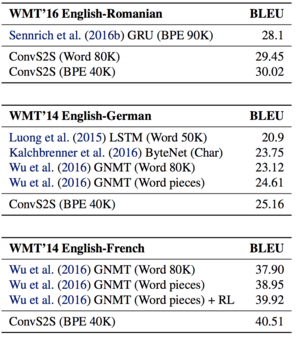
• ConvS2S outperforms the WMT’16 winning entry for English-Romanian by 1.9 BLEU with a BPE encoding and by 1.3 BLEU with a word factored vocabulary.
• The results (Result 1) show that the convolutional model outpeforms GNMT by 0.5 BLEU on WMT 14' English to German.
• Finally the model is compared to WMT '14 English to French. The model improves over GNMT in the same setting by 1.6 BLEU on average. It also outperforms their reinforcement (RL) models by 0.5 BLEU.

Result 2: Accuracy of ensembles with other ensemble models

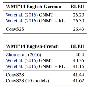
The authors ensemble eight likelihood-trained models for both WMT’14 English-German and WMT’14 English-French and compare to previous work which also reported ensemble results and find out that they outperform all the models.

Result 3 :CPU and GPU generation speed in seconds on the development set of WMT’14 English-French

Result 4 :Effect of removing position embeddings from our model in terms of validation perplexity

Result 5: Multi-step attention in all five decoder layers or fewer layers in terms of validation perplexity (PPL) and test BLEU.

Result 6: Encoder with different kernel width in terms of BLEU

Result 7: Decoder with different kernel width in terms of BLEU

Result 8: Accuracy on two summarization tasks in terms of Rouge-1 (RG-1), Rouge-2 (RG-2), and Rouge-L (RG-L)

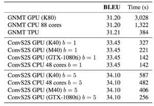
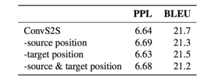
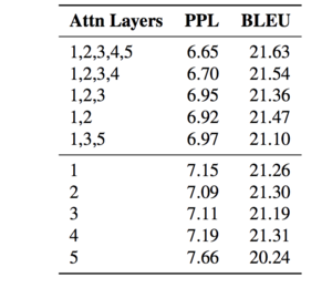
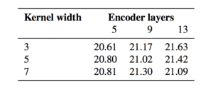
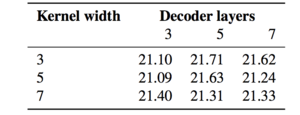
Attention for different layers

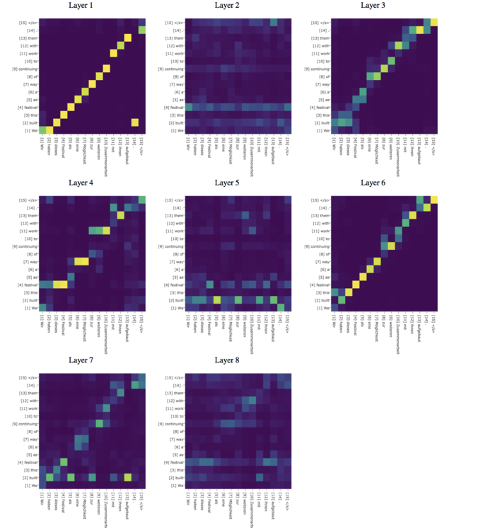
From the results of the experiments, we conclude our convolutional approach can easily discover the compositional structure in the sequences, because the representations are built hierarchically and our model relies on gating and it performs multiple attention steps. When trained with standard likelihood method, our trained CNN model outperforms the likelihood trained model (RNN MLE) which either optimize the evaluation metric, and is not far behind the best models on this task which benefit from task-specific optimization and model structure

References

1. Cho, Kyunghyun, Van Merrienboer, Bart, Gulcehre, ¨ Caglar, Bahdanau, Dzmitry, Bougares, Fethi, Schwenk, Holger, and Bengio, Yoshua. Learning Phrase Representations using RNN Encoder-Decoder for Statistical Machine Translation. In Proc. of EMNLP, 2014.
2. Bradbury, James, Merity, Stephen, Xiong, Caiming, and Socher, Richard. Quasi-Recurrent Neural Networks. arXiv preprint arXiv:1611.01576, 2016.
3. He, Kaiming, Zhang, Xiangyu, Ren, Shaoqing, and Sun, Jian. Delving deep into rectifiers: Surpassing humanlevel performance on imagenet classification. In Proceedings of the IEEE International Conference on Computer Vision, pp. 1026–1034, 2015b.
4. Meng, Fandong, Lu, Zhengdong, Wang, Mingxuan, Li, Hang, Jiang, Wenbin, and Liu, Qun. Encoding Source Language with Convolutional Neural Network for Machine Translation. In Proc. of ACL, 2015.
5. Bahdanau, Dzmitry, Cho, Kyunghyun, and Bengio, Yoshua. Neural machine translation by jointly learning to align and translate. arXiv preprint arXiv:1409.0473, 2014.
6. Gehring, Jonas, Auli, Michael, Grangier, David, and Dauphin, Yann N. A Convolutional Encoder Model for Neural Machine Translation. arXiv preprint arXiv:1611.02344, 2016.
7. Gehring et.al A Convolutional Encoder Model for Neural Machine Translation, ACL 2017
8. Dyer, Chris, Chahuneau, Victor, and Smith, Noah A. A Simple, Fast, and Effective Reparameterization of IBM Model 2. In Proc. of ACL, 2013.
9. A Short tutorial on Attention models: https://machinelearningmastery.com/attention-long-short-term-memory-recurrent-neural-networks/
10. Standford's Lecture on Neural Machine Translation and Attention Models: https://www.youtube.com/watch?v=IxQtK2SjWWM
11. https://en.wikipedia.org/wiki/BLEU
12. Papineni, K., Roukos, S., Ward, T., Henderson, J and Reeder, F. (2002). “Corpus-based Comprehensive and Diagnostic MT Evaluation: Initial Arabic, Chinese, French, and Spanish Results” in Proceedings of Human Language Technology 2002, San Diego, pp. 132–137
13. Callison-Burch, C., Osborne, M. and Koehn, P. (2006) "Re-evaluating the Role of BLEU in Machine Translation Research" in 11th Conference of the European Chapter of the Association for Computational Linguistics: EACL 2006 pp. 249–256
14. Sutskever, Ilya, Martens, James, Dahl, George E., and Hinton, Geoffrey E. On the importance of initialization and momentum in deep learning. In ICML, 2013.
15. Dauphin, Y., Fan, A., Auli, M., and Grangier, D. 2017. 'Language Modelling with Gated Convolutional Networks". ICML.
16. Shen, Shiqi, Zhao, Yu, Liu, Zhiyuan, Sun, Maosong, etal. Neural headline generation with sentence-wise optimization. arXiv preprint arXiv:1604.01904, 2016.

Implementation Example: https://github.com/facebookresearch/fairseq