dropout: Difference between revisions
(→Model) |
|
(No difference)
| |
Latest revision as of 09:46, 30 August 2017
Introduction
Dropout<ref>https://www.cs.toronto.edu/~hinton/absps/JMLRdropout.pdf</ref> is one of the techniques for preventing overfitting in deep neural network which contains a large number of parameters. The key idea is to randomly drop units from the neural network during training. During training, dropout samples from an exponential number of different “thinned” network. At test time, we approximate the effect of averaging the predictions of all these thinned networks.
By dropping a unit out, we mean temporarily removing it from the network, along with all its incoming and outgoing connections, as shown in Figure 1. Each unit is retrained with probability p independent of other units (p can be set using a validation set, or can be set to 0.5, which seems to be close to optimal for a wide range of networks and tasks).
Model
Consider a neural network with [math]\displaystyle{ \ L }[/math] hidden layer. Let [math]\displaystyle{ \bold{z^{(l)}} }[/math] denote the vector inputs into layer [math]\displaystyle{ l }[/math], [math]\displaystyle{ \bold{y}^{(l)} }[/math] denote the vector of outputs from layer [math]\displaystyle{ l }[/math]. [math]\displaystyle{ \ \bold{W}^{(l)} }[/math] and [math]\displaystyle{ \ \bold{b}^{(l)} }[/math] are the weights and biases at layer [math]\displaystyle{ l }[/math]. With dropout, the feed-forward operation becomes:
- [math]\displaystyle{ \ r^{(l)}_j \sim Bernoulli(p) }[/math]
- [math]\displaystyle{ \ \tilde{\bold{y}}^{(l)}=\bold{r}^{(l)} * \bold y^{(l)} }[/math] , here * denotes an element-wise product.
- [math]\displaystyle{ \ z^{(l+1)}_i = \bold w^{(l+1)}_i\tilde {\bold y}^l+b^{(l+1)}_i }[/math]
- [math]\displaystyle{ \ y^{(l+1)}_i=f(z^{(l+1)}_i) }[/math] , where [math]\displaystyle{ f }[/math] is the activation function.
For any layer [math]\displaystyle{ l }[/math], [math]\displaystyle{ \bold r^{(l)} }[/math] is a vector of independent Bernoulli random variables each of which has probability of [math]\displaystyle{ p }[/math] of being 1. [math]\displaystyle{ \tilde {\bold y} }[/math] is the input after we drop some hidden units. The rest of the model remains the same as the regular feed-forward neural network.
Backpropagation in Dropout Case (Training)
Dropout neural network can be trained using stochastic gradient descent in a manner similar to standard neural network. The only difference here is that we only back propagate on each thinned network. The gradient for each parameter are averaged over the training cases in each mini-batch. Any training case which does not use a parameter contributes a gradient of zero for that parameter.
Dropout can also be applied to finetune nets that have been pretrained using stacks of RBMs, autoencoders or Deep Boltzmann Machines. Pretraining followed by finetuning with backpropagation has been shown to give significant performance boosts over finetuning from random initializations in certain cases. This is done by performing the regular pretraining methods (RBMs, autoencoders, ... etc). After pretraining, the weights are scaled up by factor [math]\displaystyle{ 1/p }[/math], and then dropout finetuning is applied. The learning rate should be a smaller one to retain the information in the pretrained weights.
Max-norm Regularization
Using dropout along with max-norm regularization, large decaying learning rates and high momentum provides a significant boost over just using dropout. Max-norm constrain the norm of the incoming weight vector at each hidden unit to be upper bounded by a fixed constant [math]\displaystyle{ c }[/math]. Mathematically, if [math]\displaystyle{ \bold w }[/math] represents the vector of weights incident on any hidden unit, then we put constraint [math]\displaystyle{ ||\bold w ||_2 \leq c }[/math]. A justification for this constrain is that it makes the model possible to use huge learning rate without the possibility of weights blowing up.
Unsupervised Pretraining
Neural networks can be pretrained using stacks of RBMs<ref name=GeH> Hinton, Geoffrey, et al "Reducing the dimensionality of data with neural networks." in Science,, (2006). </ref> , autoencoders<ref name=ViP> Vincent, Pascal, et al "Stacked denoising autoencoders: Learning useful representations in a deep network with a local denoising criterion." in Proceedings of the 27th International Conference on Machine Learning,, (2010). </ref> or Deep Boltzmann Machines<ref name=SaR> Salakhutdinov , Ruslan, et al [http://www.utstat.toronto.edu/~rsalakhu/papers/dbm.pdf "Deep Boltzmann Machines ."] in Proceedings of the International Conference on Artificial Intelligence and Statistics(2009). </ref>. Pretraining is an effective way of making use of unlabeled data. Pretraining followed by finetuning with backpropagation has been shown to give significant performance boosts over finetuning from random initializations in certain cases. Dropout can be applied to finetune nets that have been pretrained using these techniques. The pretraining procedure stays the same.
Test Time
Suppose a neural net has n units, there will be [math]\displaystyle{ 2^n }[/math] possible thinned neural networks. It is not feasible to explicitly run exponentially many thinned models and average them to obtain a prediction. Thus, at test time, the idea is to use a single neural net without dropout. The weight of this network are scaled-down versions of the trained weights. If a unit is retained with probability [math]\displaystyle{ p }[/math] during training, the outgoing weights of that unit are multiplied by [math]\displaystyle{ p }[/math] at test time. Figure below shows the intuition.
Multiplicative Gaussian Noise
Dropout takes Bernoulli distributed random variables which take the value 1 with probability [math]\displaystyle{ p }[/math] and 0 otherwise. This idea can be generalized by multiplying the activations by a random variable drawn from [math]\displaystyle{ \mathcal{N}(1, 1) }[/math]. It works just as well, or perhaps better than using Bernoulli noise. That is, each hidden activation [math]\displaystyle{ h_i }[/math] is perturbed to [math]\displaystyle{ h_i+h_ir }[/math] where [math]\displaystyle{ r \sim \mathcal{N}(0,1) }[/math], which equals to [math]\displaystyle{ h_ir' }[/math] where [math]\displaystyle{ r' \sim \mathcal{N}(1, 1) }[/math]. We can generalize this to [math]\displaystyle{ r' \sim \mathcal{N}(1, \sigma^2) }[/math] which [math]\displaystyle{ \sigma^2 }[/math] is a hyperparameter to tune.
Applying dropout to linear regression
Let [math]\displaystyle{ X \in \mathbb{R}^{N\times D} }[/math] be a data matrix of N data points. [math]\displaystyle{ \mathbf{y}\in \mathbb{R}^N }[/math] be a vector of targets.Linear regression tries to find a [math]\displaystyle{ \mathbf{w}\in \mathbb{R}^D }[/math] that maximizes [math]\displaystyle{ \parallel \mathbf{y}-X\mathbf{w}\parallel^2 }[/math].
When the input [math]\displaystyle{ X }[/math] is dropped out such that any input dimension is retained with probability [math]\displaystyle{ p }[/math], the input can be expressed as [math]\displaystyle{ R*X }[/math] where [math]\displaystyle{ R\in \{0,1\}^{N\times D} }[/math] is a random matrix with [math]\displaystyle{ R_{ij}\sim Bernoulli(p) }[/math] and [math]\displaystyle{ * }[/math] denotes element-wise product. Marginalizing the noise, the objective function becomes
[math]\displaystyle{ \min_{\mathbf{w}} \mathbb{E}_{R\sim Bernoulli(p)}[\parallel \mathbf{y}-(R*X)\mathbf{w}\parallel^2 ] }[/math]
This reduce to
[math]\displaystyle{ \min_{\mathbf{w}} \parallel \mathbf{y}-pX\mathbf{w}\parallel^2+p(1-p)\parallel \Gamma\mathbf{w}\parallel^2 }[/math]
where [math]\displaystyle{ \Gamma=(diag(X^TX))^{\frac{1}{2}} }[/math]. Therefore, dropout with linear regression is equivalent to ridge regression with a particular form for [math]\displaystyle{ \Gamma }[/math]. This form of [math]\displaystyle{ \Gamma }[/math] essentially scales the weight cost for weight [math]\displaystyle{ w_i }[/math] by the standard deviation of the [math]\displaystyle{ i }[/math]th dimension of the data. If a particular data dimension varies a lot, the regularizer tries to squeeze its weight more.
Bayesian Neural Networks and Dropout
For some data set [math]\displaystyle{ \,{(x_i,y_i)}^n_{i=1} }[/math], the Bayesian approach to estimating [math]\displaystyle{ \,y_{n+1} }[/math] given [math]\displaystyle{ \,x_{n+1} }[/math] is to pick some prior distribution, [math]\displaystyle{ \,P(\theta) }[/math], and assign probabilities for [math]\displaystyle{ \,y_{n+1} }[/math] using the posterior distribution based on the prior distribution and the data set.
The general formula is:
[math]\displaystyle{ \,P(y_{n+1}|y_1,\dots,y_n,x_1,\dots,x_n,x_{n+1})=\int P(y_{n+1}|x_{n+1},\theta)P(\theta|y_1,\dots,y_n,x_1,\dots,x_n)d\theta }[/math]
To obtain a prediction, it is common to take the expected value of this distribution to get the formula:
[math]\displaystyle{ \,\hat y_{n+1}=\int y_{n+1}P(y_{n+1}|x_{n+1},\theta)P(\theta|y_1,\dots,y_n,x_1,\dots,x_n)d\theta }[/math]
This formula can be applied to a neural network by thinking of [math]\displaystyle{ \,\theta }[/math] as all of the parameters in the neural network and [math]\displaystyle{ \,P(y_{n+1}|x_{n+1},\theta) }[/math] can be thought as the output of the neural network given some set of weights and the input. Since the output of a neural network is fixed and the probability is 1 for a single output and 0 for all other possible outputs, the formula can be rewritten as:
[math]\displaystyle{ \,\hat y_{n+1}=\int f(x_{n+1},\theta)P(\theta|y_1,\dots,y_n,x_1,\dots,x_n)d\theta }[/math]
Where [math]\displaystyle{ \,f(x_{n+1},\theta) }[/math] is the output of the neural network given some weights and input. By taking a closer look at this expected values formula, it is essentially the average of infinitely many possible neural network outputs weighted by its probability of occurring given the data set.
In the dropout model, the researchers are doing something very similar in that they take the average of the outputs of a wide variety of models with different weights but unlike Bayesian neural networks where each of these outputs and their respective models are weighted by their proper probability of occurring, the dropout model assigns equal probability to each model. This necessarily impacts the accuracy of dropout neural networks compared to Bayesian neural networks but have very strong advantages in training speed and ability to scale.
Despite the erroneous probability weighting compared to Bayesian neural networks, the researchers compared the two models and found that while it is less accurate, it is still better than standard neural network models and can be seen in their chart below, higher is better:
Effects of Dropout
Effect on Features
In a standard neural network, units may change in a way that they fix up the mistakes of the other units, which may lead to complex co-adaptations and overfitting because these co-adaptations do not generalize to unseen data. Dropout breaks the co-adaptations between hidden units by making the presence of other units unreliable. Firgure 7a shows that each hidden unit has co-adapted in order to produce good reconstructions. Each hidden unit its own does not detect meaningful feature. In figure 7b, the hidden units seem to detect edges, strokes and spots in different parts of the image. File:feature.png
Effect on Sparsity
Sparsity helps preventing overfitting. In a good sparse model, there should only be a few highly activated units for any data case. Moreover, the average activation of any unit across data cases should be low. Comparing the histograms of activations we can see that fewer hidden units have high activations in Figure 8b compared to figure 8a. File:sparsity.png
Effect of Dropout Rate
The paper tested to determine the tunable hyperparameter [math]\displaystyle{ p }[/math]. The comparison is down in two situations:
 1. The number of hidden units is held constant. (fixed n)
 2. The expected number of hidden units that will be retained after dropout is held constant. (fixed [math]\displaystyle{ pn  }[/math] )
The optimal [math]\displaystyle{ p }[/math] in case 1 is between (0.4, 0.8 ); while the one in case 2 is 0.6. The usual default value in practice is 0.5 which is close to optimal. File:pvalue.png
Effect of Data Set Size
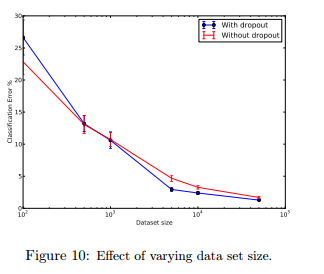
This section explores the effect of changing data set size when dropout is used with feed-forward networks. From Figure 10, apparently, dropout does not give any improvement in small data sets(100, 500). As the size of the data set is increasing, then gain from doing dropout increases up to a point and then decline.
Comparison
The same network architecture (784-1024-1024-2048-10) with ReLUs was trained using stochastic gradient descent with different regularizations. Dropout + Max-norm outperforms all other chosen methods. The result is below:
Result
The author performed dropout on MNIST data and did comparison among different methods. The MNIST data set consists of 28 X 28 pixel handwritten digit images. The task is to classify the images into 10 digit classes. From the result table, Deep Botlzman Machine + dropout finetuning outperforms with only 0.79% Error rate.
In order to test the robustness of dropout, they did classification experiments with networks of many different architectures keeping all hyperparameters fixed. The figure below shows the test error rates obtained for these different architectures as training progresses. Dropout gives a huge improvement across all architectures.
The author also apply dropout scheme on many neural networks and test on different datasets, such as Street View House Numbers (SVHN), CIFAR, ImageNet and TIMIT dataset. Adding dropout can always reduce the error rate and further improve the performance of neural networks.
Conclusion
Dropout is a technique to prevent overfitting in deep neural network which has large number of parameters. It can also be extended to Restricted Boltzmann Machine and other graphical models, eg(Convolutional network). One drawback of dropout is that it increases training time. This creates a trade-off between overfitting and training time.
Reference
<references />


